Time series-based machine learning framework for stock market forecasting

Project description


Overview
AuToMaR is a customizable time series-based machine learning framework for forecasting the stock market. Built in Python, it provides both a powerful web-based GUI and a command-line interface for financial data analysis and model training.
The framework supports sector-aware modeling: optionally extract data for all companies in a chosen economic sector, apply PCA dimensionality reduction to capture sector-wide patterns, and train models on this enriched feature space. This allows models to learn from industry-level dynamics and correlations, or work with individual stocks in isolation.
Key capabilities:
| Component | Description |
|---|---|
| Web Interface | Full-featured SvelteKit GUI with real-time job tracking and visualization |
| Data Pipeline | Yahoo Finance extraction with automated technical indicator generation |
| ML Models | GRU, Transformer, and Logistic Regression with Ray Tune hyperparameter optimization |
| Dimensionality Reduction | PCA transformation with feature name visualization |
| Validation | Growing windows cross-validation for robust time series evaluation |
| Forecasting | Multi-day ahead predictions using autoregressive feature synthesis |
| Visualization | Interactive Plotly charts with comprehensive statistical analysis |
Table of Contents
- Features
- Installation
- Quick Start
- How It Works
- Visual Tutorial
- Configuration
- Building Distribution Packages
- Requirements
- Developed With
- References
- Authors
Features
Core Operations
- Data Extraction: Fetch historical stock data from Yahoo Finance for S&P 500 companies with industry-wide feature generation
- Principal Component Analysis: Dimensionality reduction with explained variance visualization and feature importance analysis
- Hyperparameter Tuning: Distributed Ray Tune optimization with customizable search spaces
- Model Training: Train GRU, Transformer, and Logistic Regression models with full GPU support
- Cross-Validation: K-fold validation using the growing windows method for time series
- Prediction & Forecasting: Two-mode inference system:
- Evaluation Mode: Test model performance on holdout data with comprehensive metrics
- Forecast Mode: Multi-day ahead forecasting (1-30 business days) with autoregressive synthesis
System Features
- Interactive Web GUI: Full-featured interface accessible via single command (
automar gui) - Job Management: Persistent SQLite-based job tracking with filtering, progress monitoring, and result visualization
- Storage Management: Flexible path configuration with validation and per-job output customization
- CLI & Python API: Complete programmatic access for automation and scripting
- Visualization Suite: Interactive Plotly charts for training curves, confusion matrices, PCA analysis, and forecast confidence intervals
Installation
Prerequisites
Important: AuToMaR requires PyTorch, TorchEval, and Ray Tune to be installed separately due to system-specific builds (CPU vs CUDA) and platform compatibility constraints.
Windows Users: Ray Tune does not support Python 3.13 on Windows. Use Python 3.12 instead. Linux users can use Python 3.13 without issues.
Step 1 - Install PyTorch
Visit PyTorch's official installation guide and follow the instructions for your system (CPU vs CUDA, operating system).
Step 2 - Install TorchEval
pip install torcheval
Step 3 - Install Ray Tune
pip install -U "ray[data,train,tune,serve]"
See Ray's installation guide for more details.
Step 4 - Install AuToMaR
pip install automar
From Source (Development)
For development without the web interface (faster, recommended for backend development):
git clone https://codeberg.org/Kzurro/Automar.git
cd Automar

# Install dependencies first (see Prerequisites above)
# Then install automar (without web UI)
pip install -e .
This installs the package without building the web UI. You can still use all CLI commands and the API server, but the automar gui command will not be available.
Building from Source with Web UI
To build the package with the web interface included:
Prerequisites: Node.js and npm must be installed.
Linux/macOS:
git clone https://codeberg.org/Kzurro/Automar.git
cd Automar

# Install Python dependencies (PyTorch, TorchEval, Ray - see Prerequisites section)

# Build and install with web UI
BUILD_WEB=1 pip install -e .
Windows (PowerShell):
git clone https://codeberg.org/Kzurro/Automar.git
cd Automar

# Install Python dependencies (PyTorch, TorchEval, Ray - see Prerequisites section)

# Build and install with web UI
$env:BUILD_WEB=1; pip install -e .
This will install npm dependencies, build the SvelteKit frontend, and install the Python package with web UI support.
Quick Start
Web Interface (Recommended)
Start the web UI with automatic browser opening:
automar gui
This command starts the API server and automatically opens your browser to the web interface, where you can access all features through an intuitive UI.
Alternative: API server only
automar api --host 127.0.0.1 --port 8000
Then manually navigate to http://127.0.0.1:8000 in your browser.
Command Line Interface
For automation and scripting, all operations are available via CLI:
# Extract stock data for a specific ticker
automar extract --ticker AAPL --history 10y

# Perform PCA
automar pca --dataset out/data/AAPL_10y.pkl

# Run hyperparameter tuning
automar tune --ticker AAPL --model gru

# Train a model with optimized parameters
automar train --param-file out/hyper/AAPL_gru_params.toml

# Perform cross-validation
automar crossvalidate --ticker AAPL --model gru

# Make predictions with a trained model
automar predict --model-path out/models/gru/AAPL_model.pth --dataset out/data/AAPL_10y.pkl
Python API
from automar.core.models import GRUModel
from automar.core.preprocessing import loaders

# Your custom code here
How It Works
AuToMaR implements a complete time series forecasting pipeline:
- Data Extraction: Fetches stock panel data from Yahoo Finance for a target company, with optional sector-wide extraction to include all S&P 500 companies in the chosen economic sector
- Feature Engineering: Generates technical indicators following applied deep learning literature
- Dimensionality Reduction (Optional): Apply PCA to sector-wide data to capture industry-level patterns and reduce feature space while preserving variance
- Time Series Transformation: Applies WEASEL-MUSE algorithm for time series classification
- Hyperparameter Optimization: Fine-tunes models using parallel Ray Tune optimization
- Model Training: Trains GRU, Transformer, and Logistic Regression models on either individual stock data or PCA-transformed sector features
- Robust Validation: Cross-validates using the growing windows method
- Prediction: Generates forecasts in two modes:
- Evaluation: Test set performance with comprehensive metrics
- Forecast: Multi-day ahead predictions using autoregressive synthesis
- Visualization: Creates interactive Plotly charts and statistical tables
- Job Tracking: Maintains persistent job history with filtering and result access
Visual Tutorial
This section walks through the complete workflow using the web interface. All screenshots show the actual AuToMaR GUI.
Main Operation Tabs
Data Extraction
The Data Extract tab provides an interface for fetching historical stock data from Yahoo Finance. You can configure ticker selection, time periods, output formats, and sector filtering options.
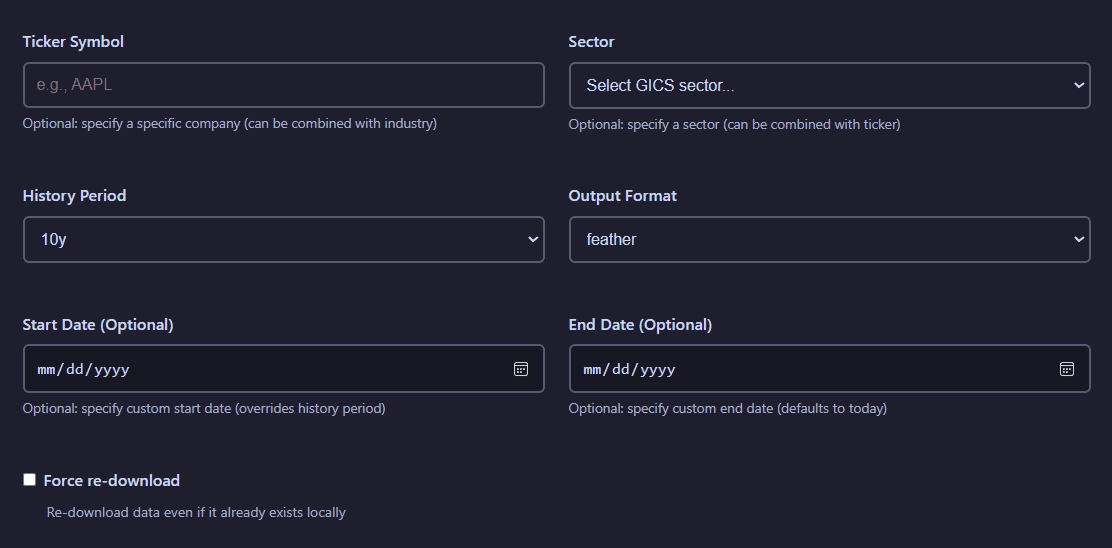
Data extraction configuration panel showing ticker selection, history period, output format, and sector filtering options
Configuration options:
- Ticker Symbol: Select from S&P 500 company ticker symbols via searchable dropdown
- Sector: Select a GICS sector whose S&P 500 companies' data will be used as context
- History Period: Choose historical data period (1y minimum, 10y maximum)
- Output Format: Export as Pickle, Feather, CSV, Excel, Parquet, or SQLite
- Start Date/End Date: Choose a range of dates to download data from, it will override the History Period settting
- Force re-download: If active, data will be downloaded even if it had been previously acquired already
View extraction results visualization
After extraction completes, the job results display a time series for the stock price evolution of the selected companies, including the plot of the mean value in the selected GICS sector.
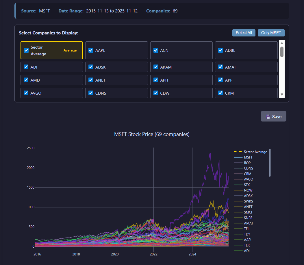
Extraction results showing the evolution of the closing stock price
Principal Component Analysis (PCA)
The PCA tab enables dimensionality reduction on your datasets. Configure the number of components, select input data sources (regular files or SQLite databases), and visualize explained variance.
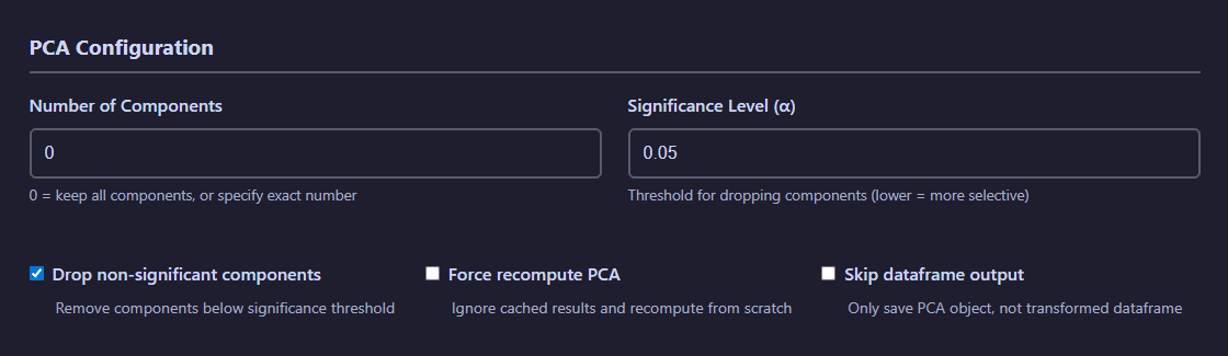
PCA configuration showing dataset selection, component count, output format, and feature visualization options
PCA Configuration:
- Number of Components: Specify target dimensionality for reduction
- Significance level: Defines threshold for the significance test
- Drop non-significant components: If active, non-significant principal components will be ignored
- Force recompute PCA: If active, PCA will be generated even if it already exists
- Skip dataframe output: If active, the transformed dataframe will not be saved
View PCA analysis visualization
PCA results include visualizations showing explained variance ratio, cumulative variance, and principal component contributions across features.
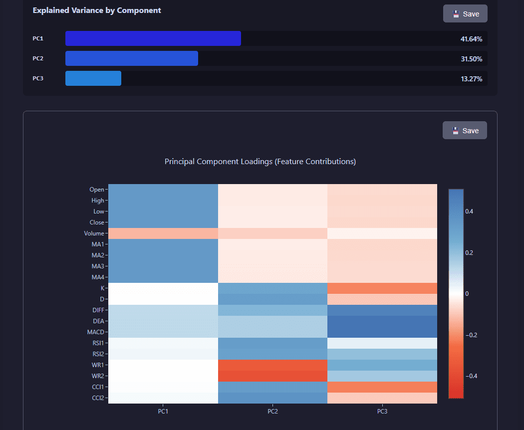
PCA analysis showing explained variance, cumulative variance, and component contributions
Hyperparameter Tuning
The Tuning tab provides Ray Tune-based hyperparameter optimization for your models. Configure search spaces, resource allocation, and the number of trials to explore.
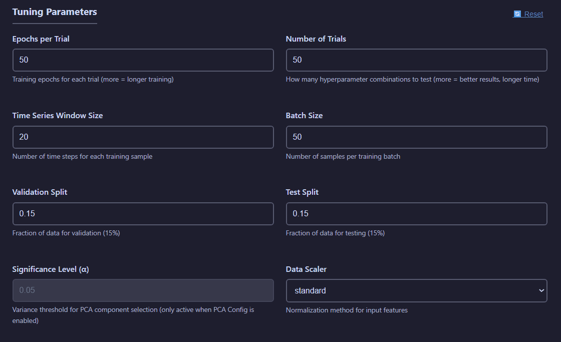
Hyperparameter tuning interface with model selection, sample count, search space configuration, and compute resources
Tuning Parameters:
- Epochs: Number of training iterations for each trial
- Number of Trials: Number of experiments to test
- Time Series Window Size: Number of observations used for each prediction
- Batch Size: Number of observations in each training batch
- Validation Split: Fraction of the total number of observations used for validation purposes
- Test Split: Fraction of the total number of observations used for testing purposes
- Significance Level: Threshold for accepting a principal component (if PCA per batch is active)
- Data Scaler: Method for data standarization to employ.
Search Space Configuration:
You can customize Ray Tune search spaces to define the hyperparameter ranges explored during optimization.
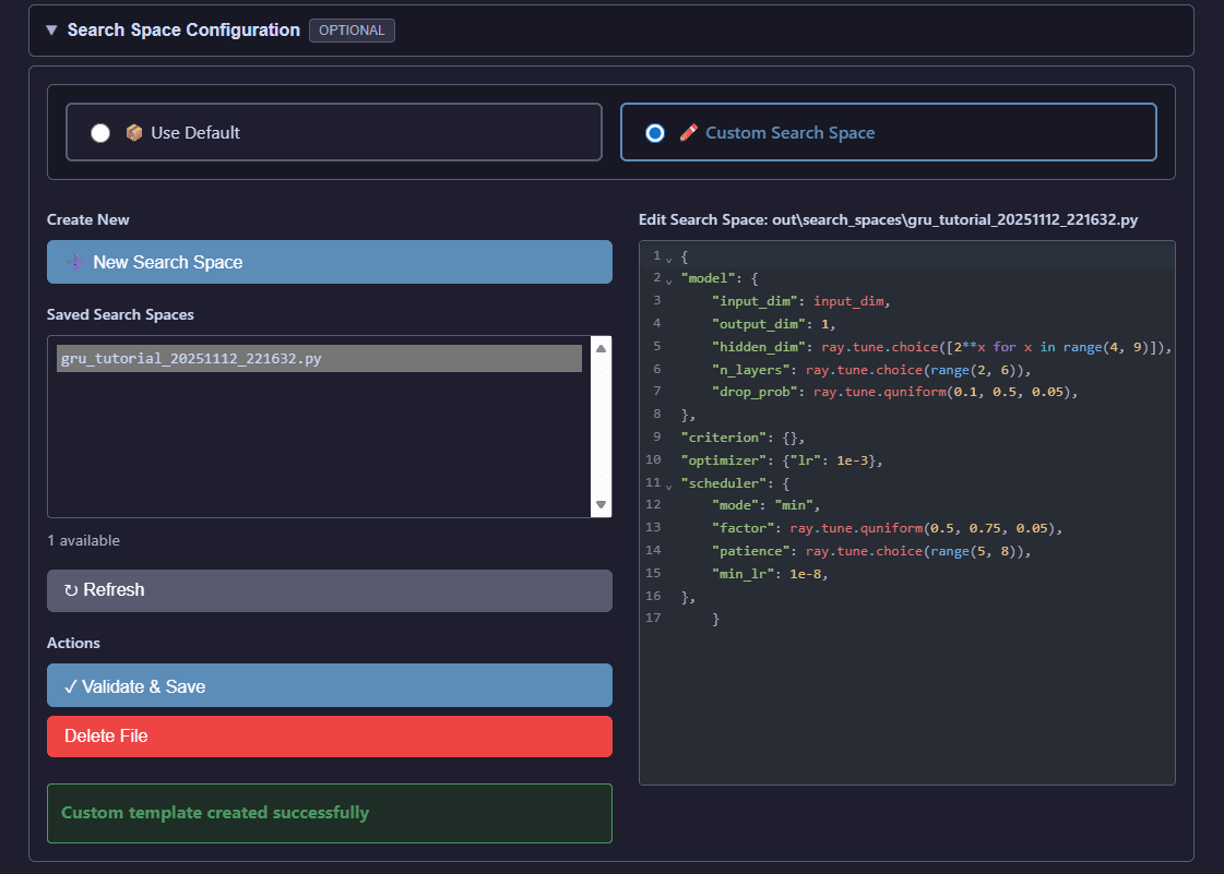
Custom search space editor for defining hyperparameter ranges and distributions
View tuning results visualization
Tuning results display Ray Tune optimization progress, showing AUROC evolution across trials, best hyperparameters found, and performance metrics.
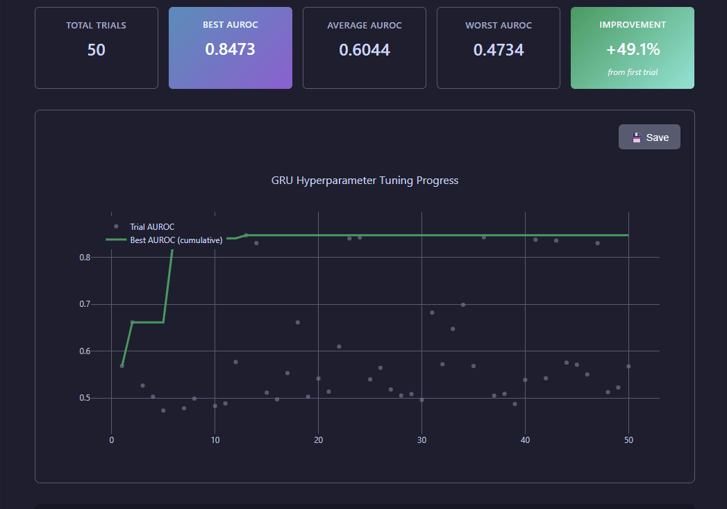
Ray Tune optimization results showing trial performance, best parameters, and convergence metrics
Model Training
The Training tab allows you to train models using optimized hyperparameters from tuning results. Configure training epochs, batch sizes, and compute resources.
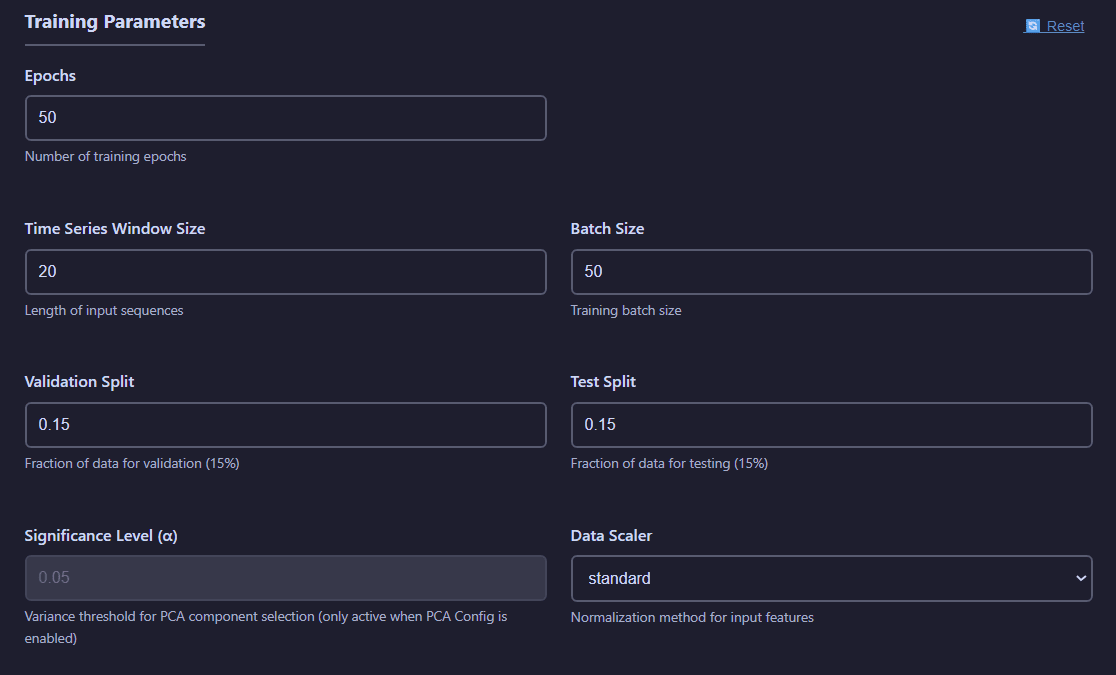
Model training configuration with hyperparameter file selection, dataset choice, and training parameters
Training Parameters:
- Epochs: Number of training iterations for each trial
- Time Series Window Size: Number of observations used for each prediction
- Batch Size: Number of observations in each training batch
- Validation Split: Fraction of the total number of observations used for validation purposes
- Test Split: Fraction of the total number of observations used for testing purposes
- Significance Level: Threshold for accepting a principal component (if PCA per batch is active)
- Data Scaler: Method for data standarization to employ.
View training visualizations
Training Loss Curves:
Inspect training and validation loss evolution throughout the training process.
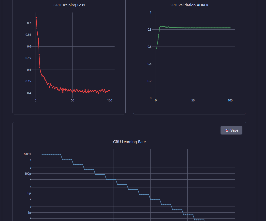
Training and validation loss curves showing model convergence over epochs
Training Metrics:
View statistics of the test for the trained model: confusion matrix and derived performance indicators.
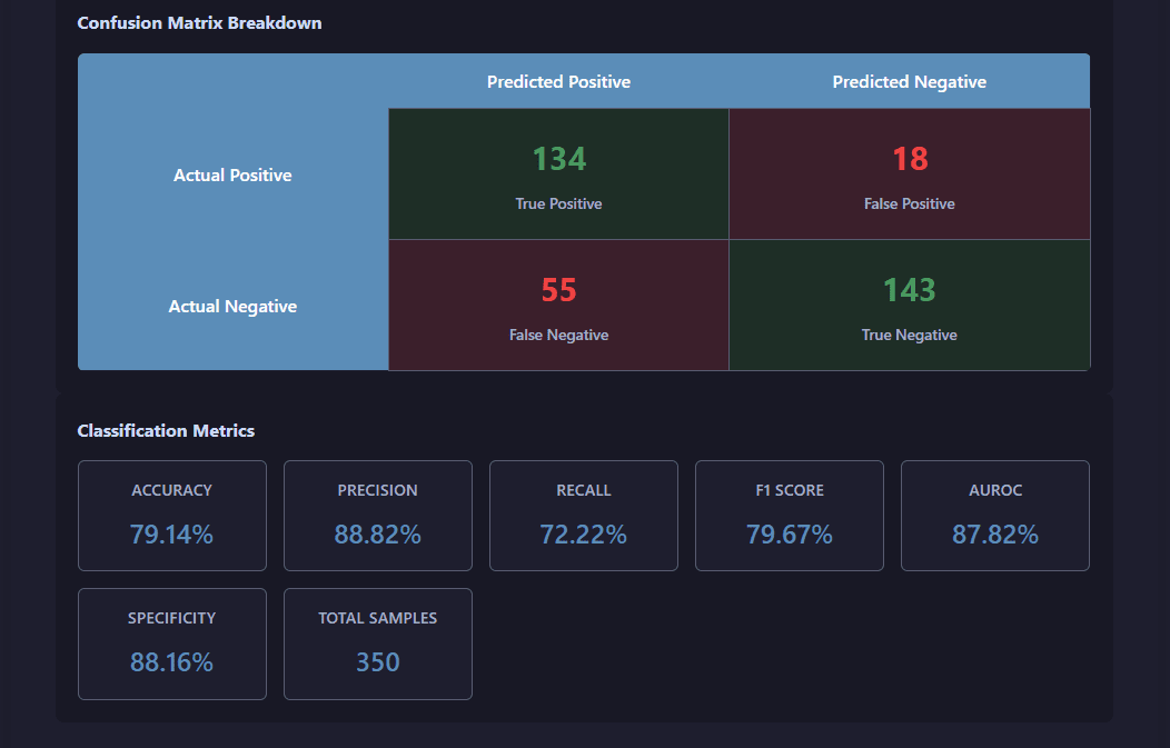
Comprehensive training metrics including AUROC, accuracy, and learning rate evolution
Cross-Validation
The Cross-Validation tab provides robust model evaluation using the growing windows method, specifically designed for time series validation.
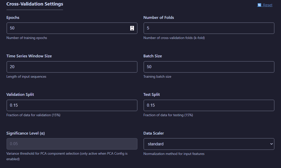
Cross-validation configuration showing fold count, model selection, and validation strategy
Cross-Validation Settings:
- Epochs: Number of training iterations for each trial
- Number of Folds: Number of growing windows models will be trained on.
- Number of Trials: Number of experiments to test
- Time Series Window Size: Number of observations used for each prediction
- Batch Size: Number of observations in each training batch
- Validation Split: Fraction of the total number of observations used for validation purposes
- Test Split: Fraction of the total number of observations used for testing purposes
- Significance Level: Threshold for accepting a principal component (if PCA per batch is active)
- Data Scaler: Method for data standarization to employ.
View cross-validation visualizations
Fold Results:
Performance metrics across all validation folds with statistical distributions.
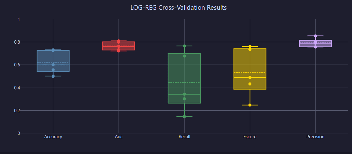
Performance metrics distribution across validation folds
Detailed Metrics:
Analyze detailed statistics and performance distributions for each fold.
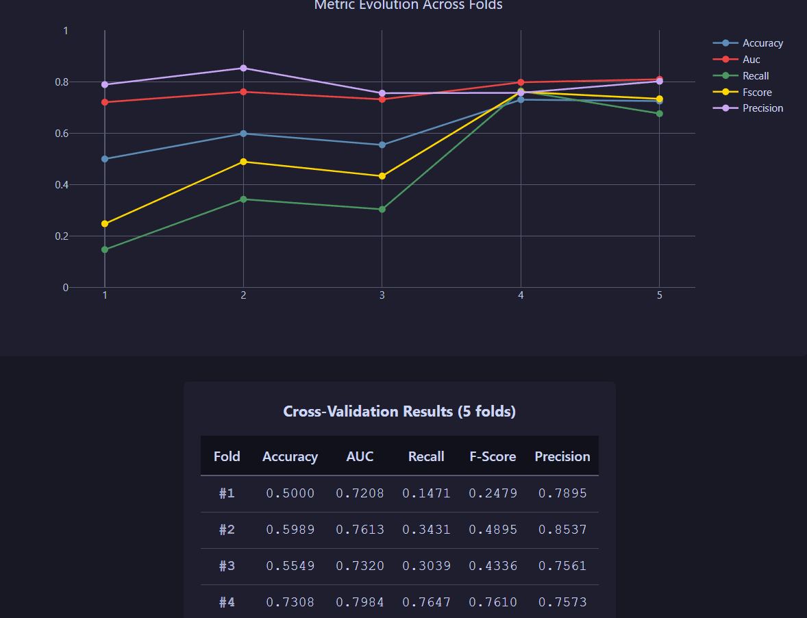
Detailed fold-by-fold performance analysis with metric breakdowns
Growing windows structure:
Distribution of available data across the requested number of folds, detailed by training, validation and test class.
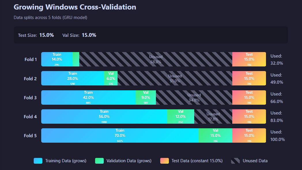
Structure of data distribution in each fold
Predictions
The Prediction tab offers model inference in two modes: Evaluation (test set performance) and Forecast (multi-day ahead predictions).
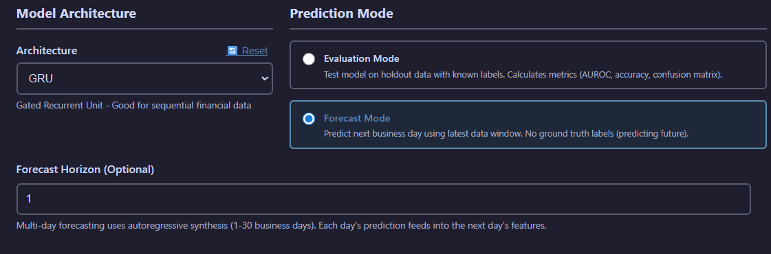
Prediction interface with mode selection, model file picker, and forecast horizon configuration
Prediction Configuration:
- Mode Selection:
- Evaluation Mode: Test model performance on holdout data with known labels
- Forecast Mode: Multi-day forecasting (1-30 business days) using autoregressive synthesis
- Forecast Horizon: Number of days ahead to predict (Forecast mode only)
View evaluation mode visualization
Evaluation mode provides comprehensive performance analysis of the pre-trained model running on the new inputted data, including the confusion matrix and classification metrics.
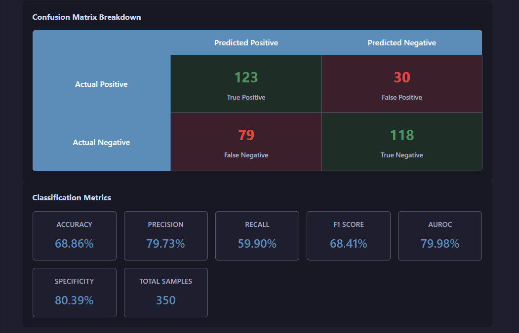
Evaluation results showing prediction accuracy, confusion matrix, and performance metrics
View forecast mode visualization
Forecast mode generates multi-day ahead predictions with confidence intervals and historical price context.
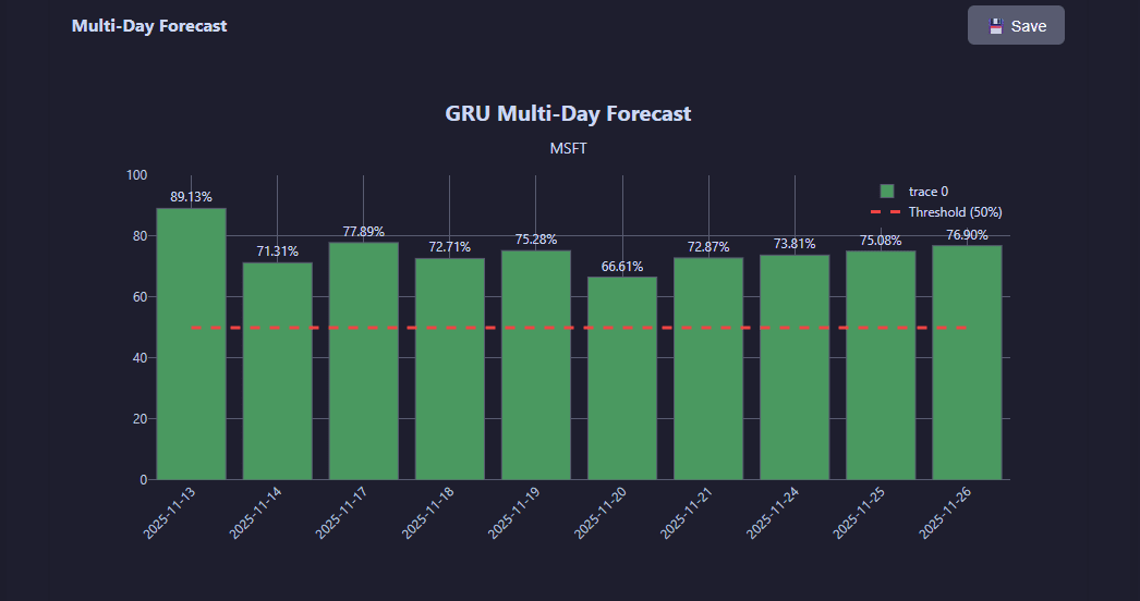
Multi-day forecast with confidence intervals, probability distributions, and historical trend context
Shared Components
The web interface includes several powerful shared components that appear across multiple operation tabs.
Data Source Selection
Choose between regular file selection and SQLite database mode with advanced filtering capabilities.
Regular File Mode:
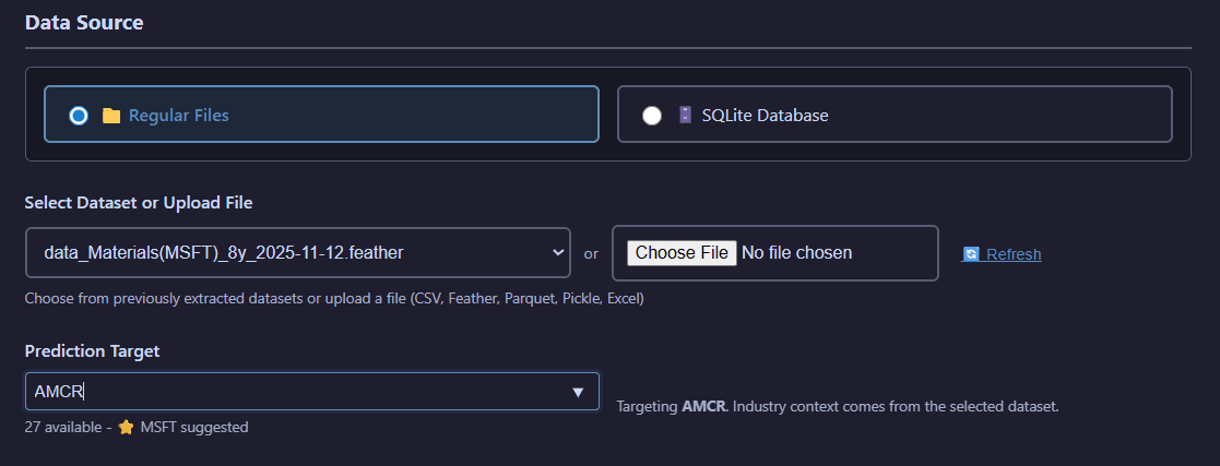
Regular file selection with ticker-specific filtering for quick dataset location
Browse and select files from the filesystem with optional ticker-based filtering to quickly find datasets for specific companies.
SQLite Database Mode:
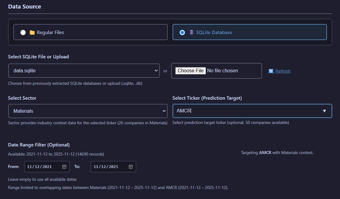
SQLite database selection with sector filtering, ticker selection, and date range controls
Query SQLite databases with advanced filtering including sector selection, target company specification, and date range constraints.
Hyperparameter Configuration
Load and manage model hyperparameters from TOML configuration files generated by tuning operations.
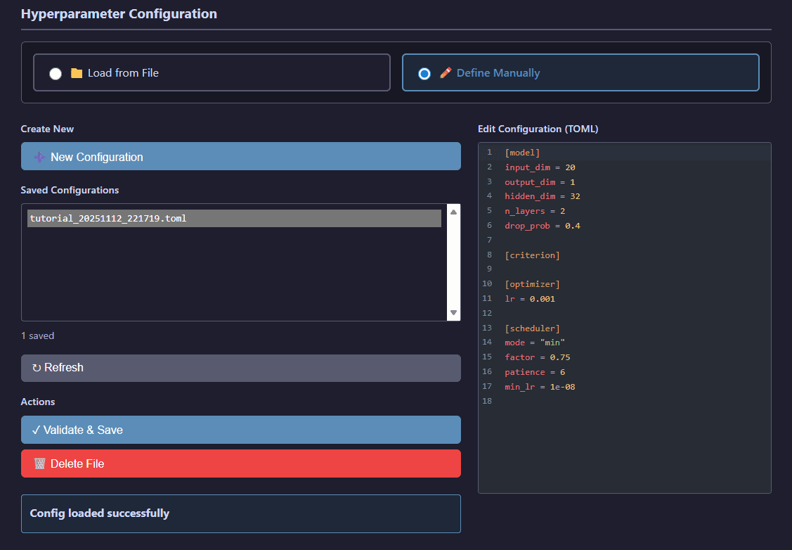
Hyperparameter file selector showing available configurations organized by model type
Browse hyperparameter configuration files organized by model architecture (GRU, Transformer, Logistic Regression) and select optimized settings from previous tuning runs.
Compute Resources
Configure CPU/GPU allocation and memory limits for computationally intensive operations.
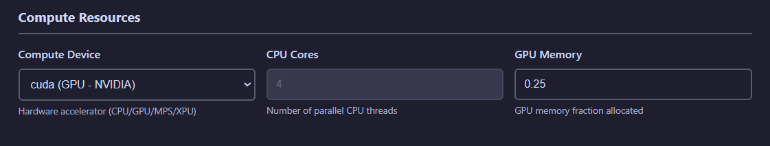
Compute resource allocation panel for device selection, CPU cores, and memory limits
Resource Configuration:
- Device: Select CPU or GPU (CUDA) execution
- CPU Cores: Number of CPU cores to utilize for parallel processing
- Memory: RAM allocation limits for data loading and processing
- GPU Memory: VRAM limits for GPU-accelerated operations
Save Location
Override default storage configuration on a per-job basis with custom output paths.
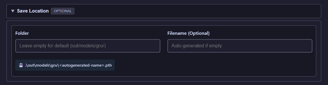
Custom save location selector for per-job output path overrides
Specify a custom output directory for individual operations, allowing you to organize results outside the default storage configuration.
System Features
Job Management
Track all operations through the persistent job management system with filtering and real-time progress monitoring.
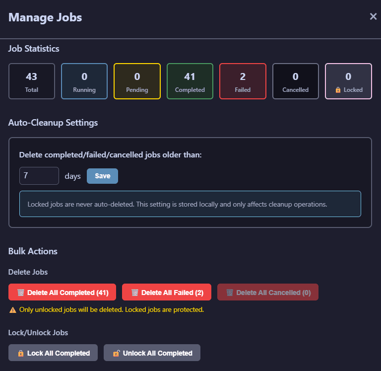
Job management panel showing active and completed jobs with filtering options
Job Management Features:
- Quantifies number of jobs in each status.
- Quick management of jobs in bulk: lock all, unlock all, delete all. Check the job card in Job Status for manipulating specific jobs.
Job Status
Access comprehensive details for individual operations including logs, parameters, and result visualizations.
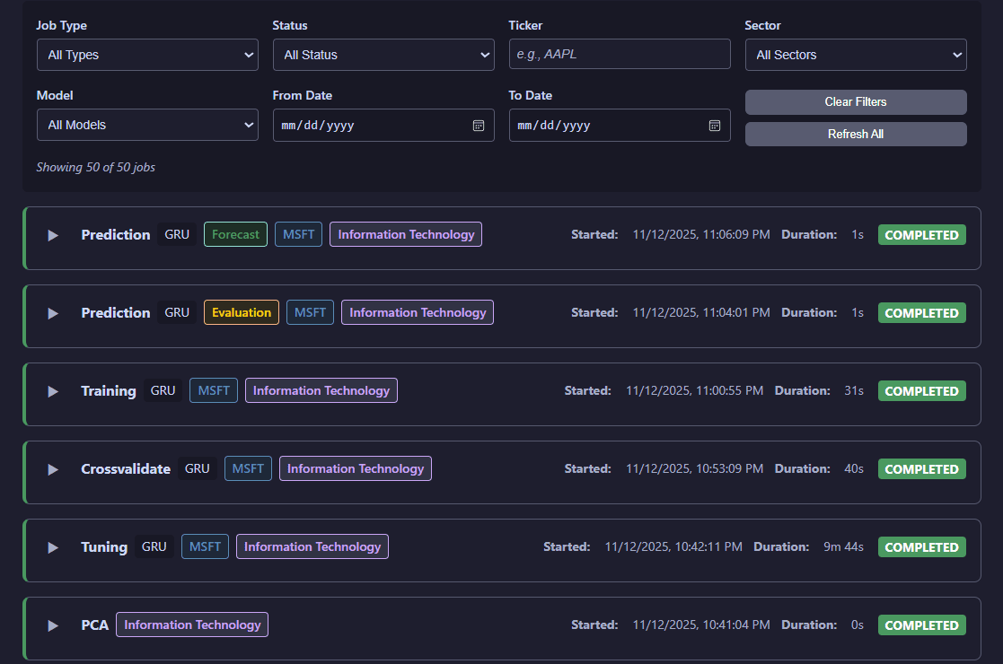
Detailed job status view with execution logs, parameters, and visualization access
Job Status Provides:
- Detailed execution logs and progress tracking
- Complete job parameters and configuration
- Output file locations and results
- Direct access to interactive visualizations for completed operations
- Status updates and error diagnostics for failed jobs
Individual Job Card:
Each job in the Job Status tab displays as an expandable card with detailed information and controls.
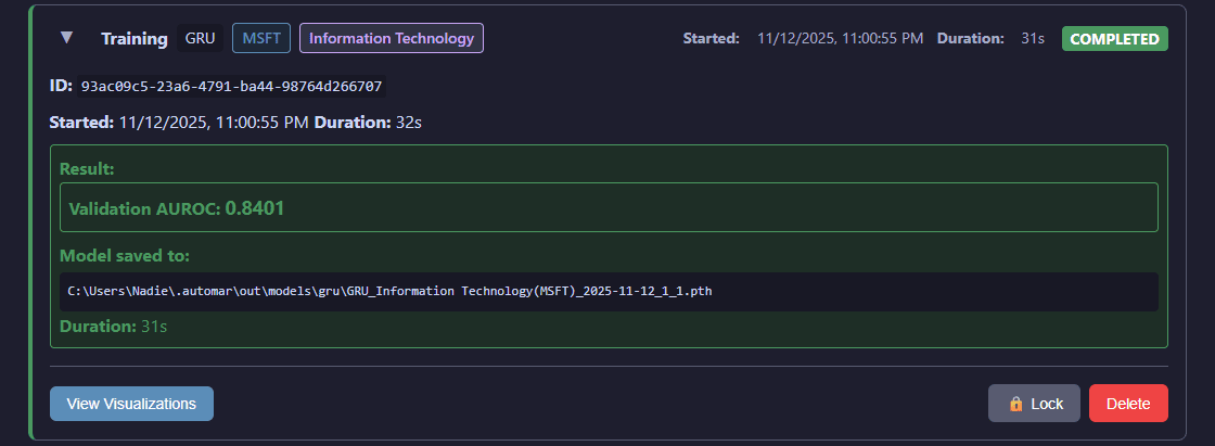
Expanded job card showing detailed information, visualization access, and management options (lock, unlock, delete)
The expanded card for each job provides quick access to the lock/unlock function (preventing both its automated and bulk deletion), delete function, and to view visualizations for succesful jobs.
Storage Configuration
Configure custom storage paths through the Settings feature accessible from the top navigation bar.
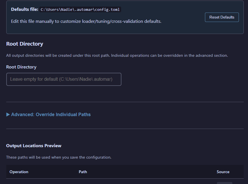
Settings interface for customizing output paths with validation
Storage Management:
- View current storage paths for all operations (data, models, PCA, predictions, etc.)
- Override root directory to change all operation paths at once
- Override individual operation paths for granular control
- Validate paths before saving to prevent configuration errors
- Changes take effect immediately without requiring server restart
Configuration
AuToMaR uses TOML configuration files for system-wide settings. A default config.toml is provided with sensible defaults. When running the web UI, these defaults are loaded directly from schema.py, then overridden by $HOME/.automar/config.toml (auto-created on first launch) before reaching the frontend. Edit that file manually to customize loader/tuning/cross-validation defaults or use the Settings modal to reset it back to schema values.
Storage Configuration
AuToMaR provides flexible path configuration with a 3-tier priority system:
- Custom paths in config.toml - Highest priority
- AUTOMAR_DATA_DIR environment variable - Medium priority
- Default location - Lowest priority (repository root or
~/.automar/)
Using the Web UI (Recommended)
The web interface includes a Manage Storage button in the top navigation bar that opens a configuration modal. You can view current paths, override the root directory or individual operation paths, validate configurations, and apply changes immediately without restarting the server.
Additionally, all operation tabs include an optional Save Location field for per-job path overrides.
Manual Configuration
Edit config.toml directly to configure storage paths:
[paths]
# Override the root directory (all operations use this as base)
root = "/custom/path/to/data"

# Or override individual operation directories
data = "/custom/path/to/datasets"
models = "/custom/path/to/models"
pca = "/custom/path/to/pca"
Environment Variable
Set the AUTOMAR_DATA_DIR environment variable to change the default storage location:
Linux/macOS:
export AUTOMAR_DATA_DIR=/path/to/custom/directory
Windows (PowerShell):
$env:AUTOMAR_DATA_DIR="C:\path\to\custom\directory"
Output Structure
Results are stored following the 3-tier path configuration priority. The default output structure within the configured location is:
out/
├── data/          # Extracted datasets (.pkl, .feather, .xlsx, .csv, .parquet, .sqlite)
├── pca/           # PCA transformations (.joblib) with feature names
│   └── data/      # PCA-transformed dataframes (.feather)
├── hyper/         # Hyperparameter configurations (.toml)
│   ├── gru/       # GRU model hyperparameters
│   ├── transformer/ # Transformer model hyperparameters
│   └── logreg/    # Logistic Regression hyperparameters
├── models/        # Trained model weights (.pth) with training context metadata
│   ├── gru/       # GRU model checkpoints
│   ├── transformer/ # Transformer model checkpoints
│   └── logreg/    # Logistic Regression model checkpoints
├── cross/         # Cross-validation results (.pkl)
├── preds/         # Prediction results (.pkl, .json)
│   ├── eval/      # Evaluation mode predictions with metrics
│   └── forecast/  # Forecast mode predictions (multi-day)
├── jobs/          # Job tracking database (.db)
├── ray/           # Ray Tune trial reports
└── search_spaces/ # Custom search spaces for tuning (.py)
Building Distribution Packages
To create distribution packages (wheels) for PyPI or local distribution:
Without Web UI (API and CLI only - smaller package):
python -m build
With Web UI (includes compiled frontend - recommended for end users):
Linux/macOS:
BUILD_WEB=1 python -m build
Windows (PowerShell):
$env:BUILD_WEB=1; python -m build
This creates:
dist/automar-*.tar.gz- Source distributiondist/automar-*-py3-none-any.whl- Wheel distribution
The wheel can be installed with pip install dist/automar-*.whl
Note: Building with
BUILD_WEB=1requires Node.js and npm installed. The build process takes longer (~30-60 seconds extra) but creates a complete package with the web UI ready to use.
Requirements
- Python >= 3.12 (Python 3.13 not supported on Windows due to Ray Tune compatibility)
- PyTorch 2.4.0+
- TorchEval 0.0.7+
- Ray Tune 2.34.0+
- See pyproject.toml for complete dependency list
Developed with
- Python 3.12
- PyTorch 2.4.0
- Scikit-Learn 1.5.1
- Sktime 0.31.0
- Ray Tune 2.34.0
- SvelteKit 1.20.4
- Plotly.js
References
Zhao, J., Zeng, D., Liang, S., Kang, H., & Liu, Q. (2021). Prediction model for stock price trend based on recurrent neural network. Journal of Ambient Intelligence and Humanized Computing, 12(1), 745-753. https://doi.org/10.1007/s12652-020-02057-0
Authors
- Alejandro Gil (Kzurro)
- Sergio Pablo-García
Release history Release notifications | RSS feed


Download files
Download the file for your platform. If you're not sure which to choose, learn more about installing packages.
Source Distribution
Built Distribution
Filter files by name, interpreter, ABI, and platform.
If you're not sure about the file name format, learn more about wheel file names.
Copy a direct link to the current filters
File details
Details for the file automar-26.6.22.tar.gz.
File metadata
- Download URL: automar-26.6.22.tar.gz
- Upload date:
- Size: 2.0 MB
- Tags: Source
- Uploaded using Trusted Publishing? No
- Uploaded via: twine/6.2.0 CPython/3.13.7
File hashes
| Algorithm | Hash digest | |
|---|---|---|
| SHA256 |
63a690ea9657f9973a4124a10d7d66c89b6c251868c48eb014d1d0a14dacc14f
|
|
| MD5 |
f243da13f110ed3402f426ac625fc9f4
|
|
| BLAKE2b-256 |
763f1623e1dc7e64d1045054b882ca54302dde47eb59b21fc07f14cb215ae480
|
File details
Details for the file automar-26.6.22-py3-none-any.whl.
File metadata
- Download URL: automar-26.6.22-py3-none-any.whl
- Upload date:
- Size: 2.0 MB
- Tags: Python 3
- Uploaded using Trusted Publishing? No
- Uploaded via: twine/6.2.0 CPython/3.13.7
File hashes
| Algorithm | Hash digest | |
|---|---|---|
| SHA256 |
681b260bbe3473ebf2f11b890e25f950e3b521b2ef9d68c39a069db0f1bd1df1
|
|
| MD5 |
c7879a17c3a9c4ddb0ffddf661ffb8e1
|
|
| BLAKE2b-256 |
67a43de2e0e2d19f68c9f8536114c06e26c34b3b50d70fa7a371d948e3fc76eb
|


