Pipeline for extracting photometry from wide-field night sky images

Project description


⭐ Star us on GitHub — it motivates us a lot!
Table of Contents
🚀 About
AutoWISP is a software pipeline for extracting high-precision photometry from astronomical observations, with special features designed for consumer-grade color cameras (e.g., DSLRs). Developed to empower citizen scientists, AutoWISP provides a complete, automated workflow from raw images to science-ready light curves, enabling transformative contributions to time-domain astronomy.
It adheres to high standards of flexibility, reusability, and reliability, utilizing well-known software design patterns, including modular and hexagonal architectures. These patterns ensure the following benefits:
-
Modularity: Different parts of the package can function independently, enhancing the package's modularity and allowing for easier maintenance and updates.
-
Testability: Improved separation of concerns makes the code more testable.
-
Maintainability: Clear structure and separation facilitate better management of the codebase.
📝 How to Install
AutoWISP is a Python 3 package. The core AstroWISP components are pre-compiled for all major operating systems (Windows, macOS, Linux) and included in the distribution.
Use the package manager pip to install AutoWISP.
pip install autowisp
📚 Documentation
To better understand the AutoWISP pipeline, we recommend visiting our Documentation site. There, you will find useful information about the individual steps, database, and/or browser-user-interface (currently under development).
Briefly, the image processing pipeline steps and their products are shown. The arrows indicate the products of each step and where they will be used.:
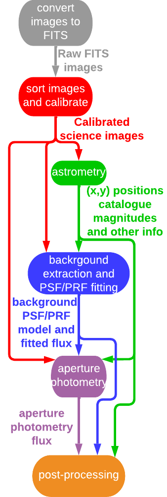
The general procedures are as follows:
Calibration
Users input their raw fits images (flat, dark, bias, or object image types as specified from their fits headers). These images are then pre-processed, where master calibration frames are generated, then frames are calibrated with these masters. This is a similar implementation as used by the HATNet, HATSouth, and HATPI projects.
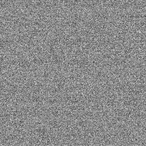
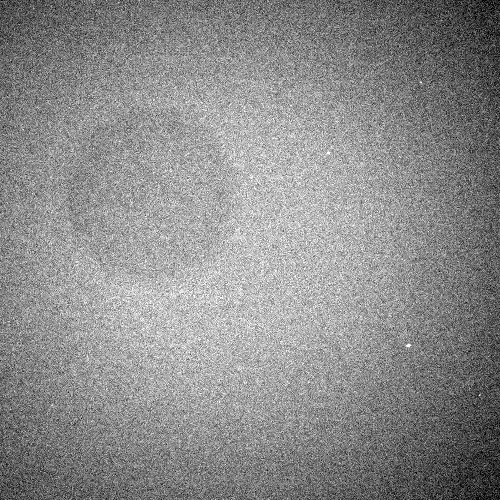
Here are example dark, flat, bias, object frames (in order as listed) gathered from a Sony-α7R DSLR Camera:
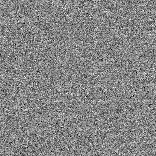
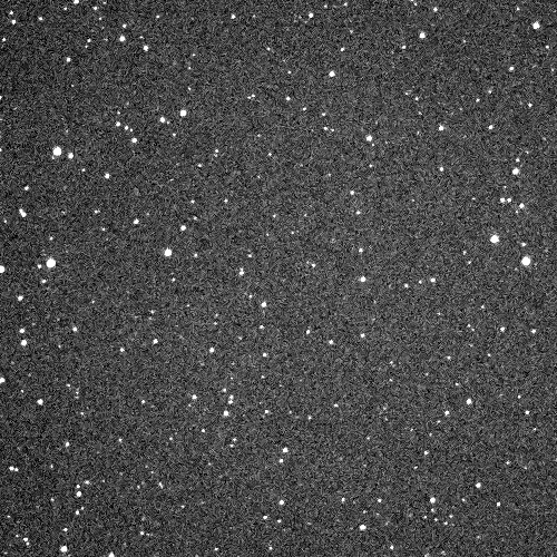
The overall calibration for object frames is given by $C(I)= \frac{I - O(I) - B_0 - (\frac{\tau[I]}{\tau[D_0]})D_0}{F_0/||F_0||}$.
Where $I$, $O(I)$, and $C(I)$ represent the image, over-scan region, and calibrated image respectively; $B_0$, $D_0$, and $F_0$ represents masters calibration images of bias, dark, and flat respectively; $\tau[I]$ and $\tau[D_0]$ are the exposure times of the image and dark frame respectively. These master frames are stacks of individually calibrated bias, dark, and flat frames. As a result, their signal-to-noise ratio is significantly increased compared to individual unstacked frames, allowing for much better calibration
Source Extraction
After the pre-processing, we extract the source (star) positions from the images and perform astrometry (plate-solving) to find a transformation that allows us to map sky coordinates (RA, Dec) into image coordinates. This allows the use of external catalogue data for more precise positions of the sources than can be extracted from survey images and the use of auxiliary data provided in the catalogue about each source in the subsequent processing steps of the pipeline.
Astrometry
Next, for each calibrated object frame, we extract flux measurements, background level, and uncertainties for the catalogue sources found in the image, which map to some position within the frame using the astrometric transformation derived in the previous step. This step is performed using AstroWISP, and we refer the reader to that article for a detailed description. We briefly summarize the process here for completeness.
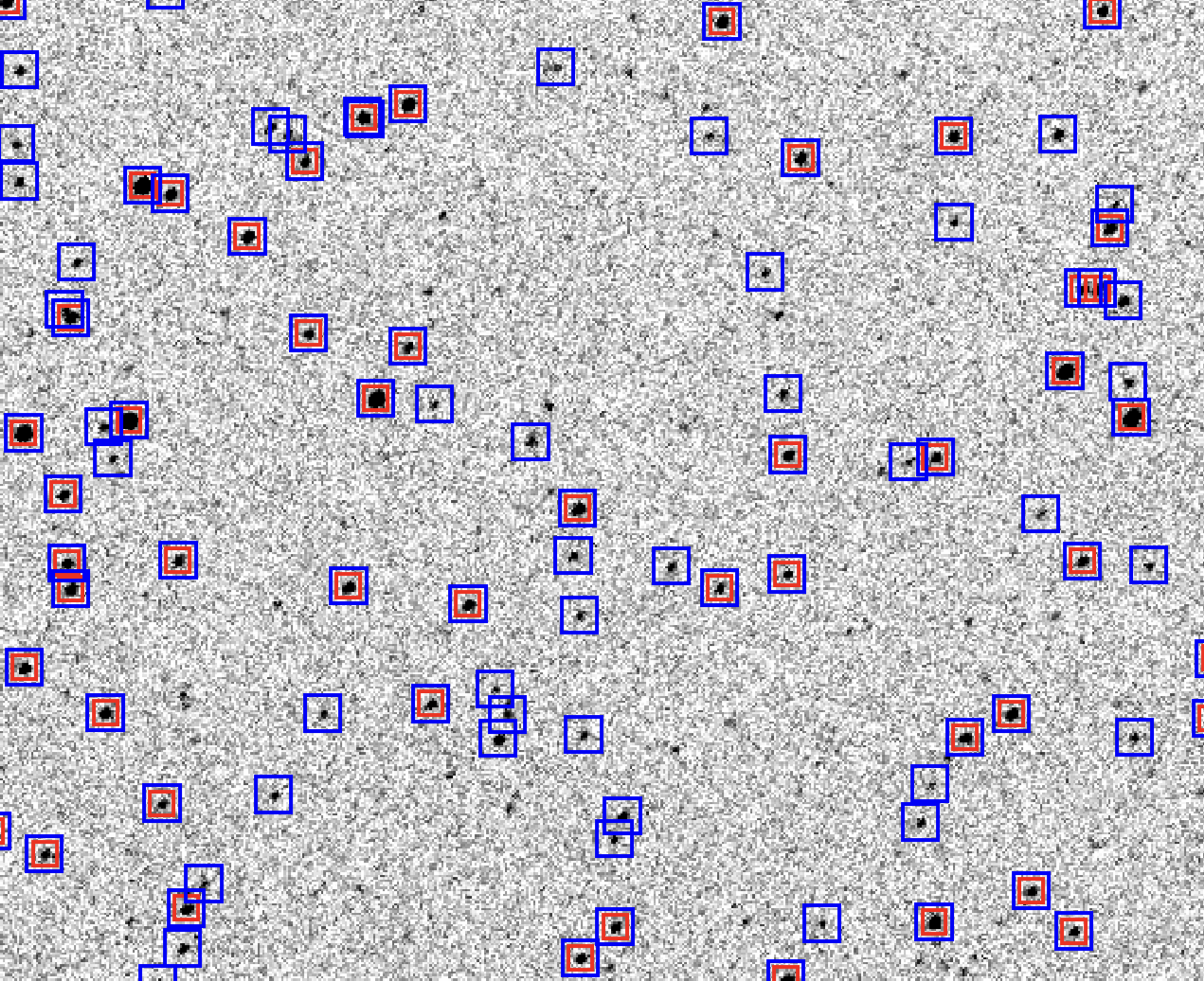
Shown is the source extraction versus catalogue projections of our astrometry step placed on top of the corresponding FITS image, where blue squares are the catalogues projected sources and red squares are the extracted sources from our astrometry
Photometry
AutoWISP takes into account the response of the pixels due to the fact that the same amount of light falling on one part of the pixel is likely to produce a different response in a different part of the pixel, this is what we call sub-pixel sensitivity. Non-uniform sensitivity on a sub-pixel level affects the PRF in an image, and the effect depends on where within a pixel the center of the source lies. Thus, it is necessary to correct for the sub-pixel sensitivity variations when deriving PSFs for a given image. For example, for DSLR or color images, we can consider the Bayer mask, which is a filter that is superimposed on the detector with arrangement of pixels sensitive to different colors in super-pixels. Since each color accounts for 1/4th of the super-pixel, the Bayer mask is an extreme version of the varying amount of the sub-pixel sensitivity. When processing a singular color channel, 3/4th of the pixel area can be considered completely insensitive to light.
There are many flavors of photometry. This pipeline supports: point spread function (PSF) or pixel response function (PRF) fitting (where the PRF is the PSF convolved with the sub-pixel sensitivity), and aperture photometry, with aperture photometry requiring PSF fitting.
PSF Fitting:
For each point source, we first measure the distribution of light on the detector (the PSF). The idea of PSF fitting is to model that distribution as some smooth parametric function centered on the projected source position with an integral equal to 1. The flux of the source is then found from a least squares scaling between the predicted and observed pixel values. While the flux will differ for each star, the shape parameters are assumed to vary smoothly as a function of source properties and position within the image. In principle, smooth changes can also be imposed across images, though that requires a highly stable observing platform in practice. For our implementation, we also take the sub-pixel sensitivity into account due to the non-uniform sensitivity of the sub-pixel level as previously described. Lastly, we store the PSF information for later use during aperture photometry.
PRF Fitting:
Similar to the PSF, we can perform PRF fitting. The PRF can be thought of as a super-resolution image of the light of a star falling on the individual pixels, where it is represented as a continuous piecewise polynomial function of sub-pixel position on each pixel (i.e., the PSF convolved with the sub-pixel sensitivity).
Aperture Photometry:
After PSF fitting, we perform aperture photometry, a photometry method that sums the flux within a circular aperture centered on each source. For aperture photometry, we correct for non–uniform pixels by using the sub-pixel sensitivity information/map and adequately integrate the PSF model to determine the fractional contributions of pixels straddling the aperture boundary.
Magnitude Fitting
After extracting flux measurements, we perform ensemble magnitude fitting. The photometry of individual frames is calibrated to the photometry of a reference frame by applying a correction as a smooth function of image position, brightness, color, and other user-specified parameters. This procedure excludes stars showing significantly larger variability than other similarly bright stars and is repeated multiple times, where the reference frame is replaced with a stack of many frames corrected in the previous iteration.
Light Curve Generation
Next, we create light curves. This is a transpose operation, collecting the photometry of each star from all images and putting them in a single file (the light curve) (see Demonstration for an example light curve)
Post Processing
Finally, after producing light curves, we perform post-processing using external parameter decorrelation (EPD) and trend filtering algorithm (TFA) to correct effects not corrected during magnitude fitting, further improving photometric precision.
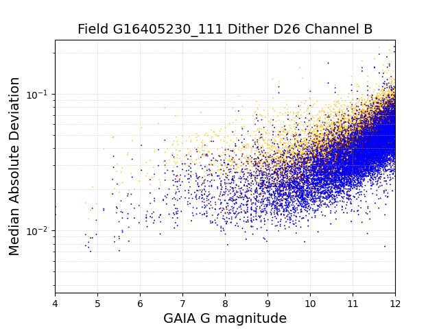
Here we show the overall improvement from our post-processing steps for the Sony-α7R DSLR Camera dataset used:
The scatter (median absolute deviation from the median (MAD)) of the individual channel light curves vs. GAIA G magnitude before EPD (only magnitude-fitting) (indicated by yellow points), after EPD but before TFA (indicated by purple points), and after TFA (indicated by their corresponding channel color (B (blue), G1 (green), G2 (green), R (red)) points).

⚙️ Demonstration
For a hands-on example, you can explore our Jupyter Notebook which processes a test dataset from start to finish.
View the interactive Processing Example on GitHub or View the interactive Processing Example on nbviewer.
This interactive notebook provides a practical demonstration of the AutoWISP pipeline in action, going step by step in the pipeline, producing the corresponding files needed for each step and ultimately creating light curves using a test dataset we provide.
[!IMPORTANT] All the following images were created using tools in this repository.
Example Light Curves
This is the resulting phase-folded lightcurve for WASP-33 b exoplanet transit, observed by Project PANOPTES (blue points and circles), TESS (red points), and theoretical light curve based on best known system parameters (green curve). The raw PANOPTES-DSLR measurements, originating from the 4 color channels of 4 cameras in Hawaii (Mauna Loa observatory) and California (Mt Wilson) are shown as blue points. The blue points are binned in time to create the blue circles and corresponding error bars. Note that the scatter in TESS points is not instrumental, but rather it is intrinsic variability in the host star, which is a member of the delta-Scuti class of variable stars.
Example Photometric Precision
The scatter (median absolute deviation from the median) of the individual channel lightcurves of PANOPTES observations of a $10\times15$ degree field centered on FU Orionis, with each of their corresponding image colors (RGGB). We see that AutoWISP enables a few parts per thousand photometric precision per exposure even from images with Bayer masks, significantly outperforming prior efforts. Even individual color channels result in better than 1% photometry per 2 min exposure.
🤝 Feedback and Contributions
We've made every effort to implement all the main aspects of AutoWISP in the best possible way. However, the development journey doesn't end here, and your input is crucial for our continuous integration and development.
[!IMPORTANT] Whether you have feedback on features, have encountered any bugs, or have suggestions for enhancements, we're eager to hear from you. Your insights help us make the AutoWISP package more robust and user-friendly.
Please feel free to contribute by submitting an issue or joining the discussions. Each contribution helps us grow and improve.
We appreciate your support and look forward to making our pipeline even better with your help!
📃 License
This package is distributed under the MIT License. You can review the full license agreement at the following link: MIT.
This package is available for free!
🗨️ Contacts
For more details about our usages, services, or any general information regarding the AutoWISP pipeline, feel free to reach out to us. We are here to provide support and answer any questions you may have. Below are the best ways to contact our team:
- Email: Send us your inquiries or support requests at support_autowisp@gmail.com.
We look forward to assisting you and ensuring your experience with AutoWISP is successful and enjoyable!
Release history Release notifications | RSS feed


Download files
Download the file for your platform. If you're not sure which to choose, learn more about installing packages.
Source Distribution
Built Distribution
Filter files by name, interpreter, ABI, and platform.
If you're not sure about the file name format, learn more about wheel file names.
Copy a direct link to the current filters
File details
Details for the file autowisp-1.0.19.tar.gz.
File metadata
- Download URL: autowisp-1.0.19.tar.gz
- Upload date:
- Size: 40.6 MB
- Tags: Source
- Uploaded using Trusted Publishing? No
- Uploaded via: twine/6.2.0 CPython/3.10.12
File hashes
| Algorithm | Hash digest | |
|---|---|---|
| SHA256 |
b67f7a3903fd3db9cdc1444bf436370cad71a7f108e09ce50d3327e6e99e31a4
|
|
| MD5 |
cfdd5ac8bb209b3906ca4e7495f77924
|
|
| BLAKE2b-256 |
4c40803c0a538b45df77159b17f60ced3b45acdf999914db5e97202be9313a24
|
File details
Details for the file autowisp-1.0.19-py3-none-any.whl.
File metadata
- Download URL: autowisp-1.0.19-py3-none-any.whl
- Upload date:
- Size: 661.2 kB
- Tags: Python 3
- Uploaded using Trusted Publishing? No
- Uploaded via: twine/6.2.0 CPython/3.10.12
File hashes
| Algorithm | Hash digest | |
|---|---|---|
| SHA256 |
c16dd0721cd8604a3a14b9aafbcf5aa35cf1fa014d849602d64c5467be224cf0
|
|
| MD5 |
e57746e3a75936d9db74efbc51bcd627
|
|
| BLAKE2b-256 |
57e09675e265273461429a77c74824f4b1bf30281c82449a4e3694e421e38ca6
|


