

aws-analyzer
Understand your AWS data from a SageMaker notebook.
One Python file per AWS service. Drop it next to your notebook and get readable reports on your S3 buckets, DynamoDB tables, Bedrock knowledge bases and the SageMaker notebook itself: what's there, what it costs, and what to do next. And a chat window for asking a knowledge base, with every setting in reach.






Guides · Get started · S3 · DynamoDB · Bedrock Knowledge Bases · Knowledge base chat · SageMaker · Development
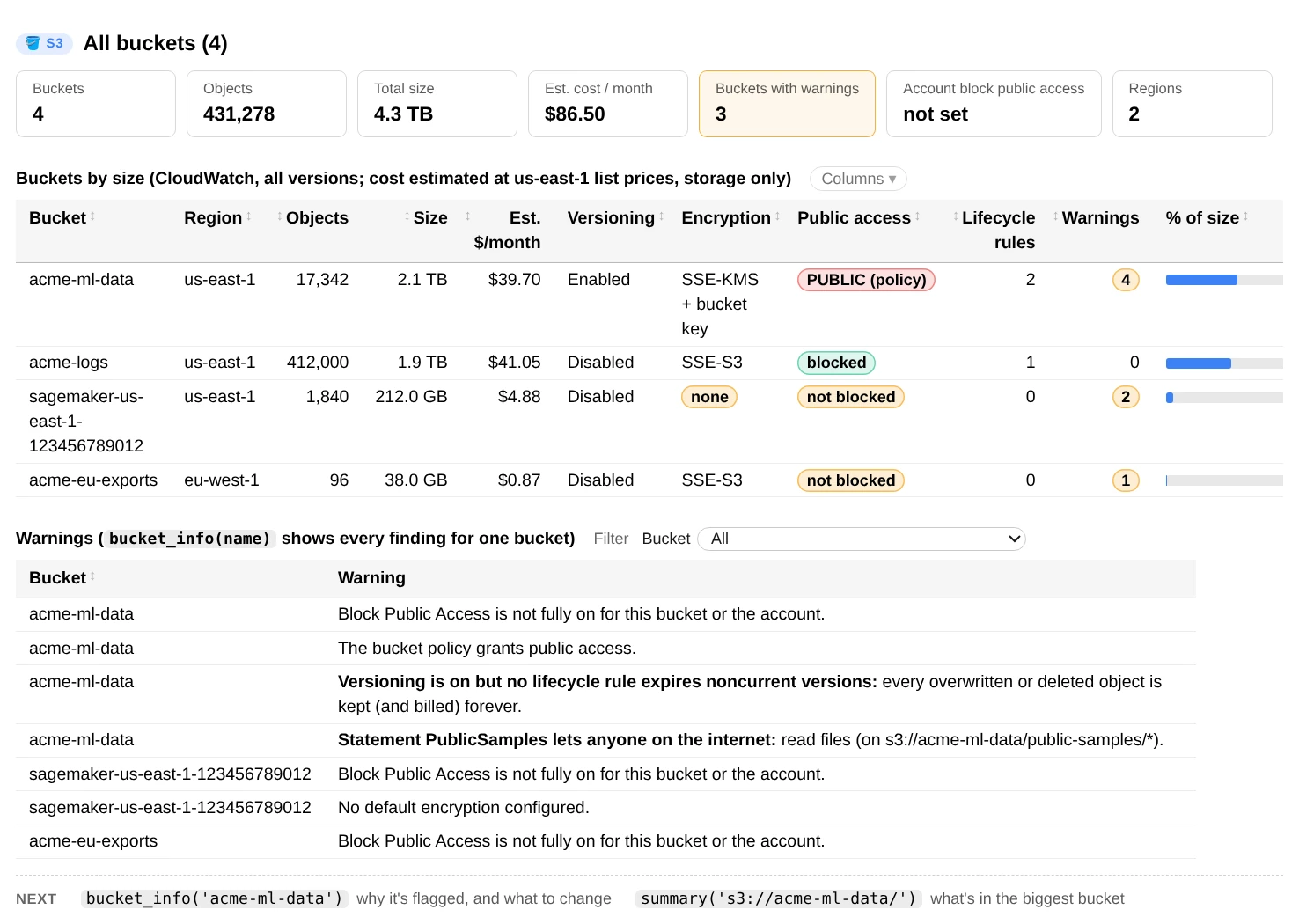
ui.overview(): every bucket's size, estimated monthly cost and security settings, what's wrong with each, and what to run next.
Why aws-analyzer
|
🧭 The answer first Each report starts with the few numbers that matter, then explains the rest in plain English: bucket policies, lifecycle rules, knowledge base settings. The raw JSON is still there, folded away. |
💵 Findings you can act on Each warning says what's wrong, why it matters and what it costs ("costing $12.40/month"), then the next step. Reports end with the commands worth running next, arguments filled in. |
🧾 Honest about cost Estimates are labelled as estimates, with the prices used. Expensive scans stop early by default and say so, and show what they read or cost. |
|
📄 One file, boto3 only Copy one file next to your notebook (no file depends on another), or pip install aws-analyzer. pandas,
pyarrow and the rest are optional.
|
🔒 Read-only Nothing writes to a bucket, table or knowledge base. Where a change would help, the report shows the command (a restore, a sync, a lifecycle rule) instead of running it. |
💬 Notes, not tracebacks A missing permission, package or broken file becomes a short note that says how to fix it, and the rest of the report still renders. |
Services
| Service | What it shows you | File and guide |
|---|---|---|
| Amazon S3 | • Every bucket's size, monthly cost and risks • Click through folders like a file explorer, or search them • Preview CSV, Parquet, JSON, Excel, PDF, Word and more • Cut storage costs and recover deleted files |
s3.py, s3_explorer.pyGuide → |
| Amazon DynamoDB | • Every table's key, size, billing and cost • Scan, query and get items as plain tables • Which attributes the items hold, and their types • The read units each report used; scans stop early |
dynamodb.pyGuide → |
| Amazon Bedrock Knowledge Bases | • Settings in plain English, sync health and failed documents • Search with sources, pages and highlighted passages • Answers with each claim linked to its source • Compare search settings and measure retrieval hit rate |
bedrock_kb.pyGuide → |
| Bedrock knowledge base chat | • A chat window: pick the knowledge base and the model • Answers stream in, with citations, sources, request and response • Add, change or remove any RetrieveAndGenerate setting • The request as highlighted JSON you can edit, or as Python |
bedrock_chat.pyGuide → |
| Amazon SageMaker | • The notebook you're in: type, cost so far, idle shutdown • Its CPU, memory, disk and GPU use right now • What fills the disk, and what's safe to clear • Everything running and billing in the region, and what looks forgotten |
sagemaker_env.pyGuide → |
The guides walk through each service with screenshots: setting up in
SageMaker, every command, and ready-made IAM policies. Their source is in docs/.
Get started
1. Install it, or put the file next to your notebook. Pick whichever works where you are:
- Install it with pip, in a notebook cell:
%pip install aws-analyzer. That's every service, and only needs boto3;%pip install "aws-analyzer[all]"also installs every optional package (pandas, pyarrow, the PDF and Excel readers, progress bars). Then import fromaws_analyzerinstead of from the file (step 2). - Upload it: download
analyzers/s3.pyand drag it into JupyterLab's file browser, in the same folder as your notebook. - Fetch it from a cell, if the notebook can reach the internet:
!curl -sO https://raw.githubusercontent.com/utkarsh5026/aws-analyzer/main/analyzers/s3.py
- Copy it from S3, for a notebook with no internet access (VPC-only mode): upload it to a bucket once, then run
!aws s3 cp s3://your-bucket/tools/s3.py . - Or paste the whole file into a notebook cell and run it.
2. Import it and look around. It uses the notebook's IAM execution role, so there's nothing to configure:
from s3 import S3View  # or DynamoDBView from dynamodb, BedrockKBView from bedrock_kb, SageMakerView from sagemaker_env
# installed with pip: from aws_analyzer import S3View (or DynamoDBView, BedrockKBView, SageMakerView, S3Explorer, chat)

ui = S3View()          # uses the notebook's IAM role
ui.help()              # every command, grouped by task; ui.help("summary") shows one in full
ui.overview()          # every bucket: size, monthly cost, security warnings
s3 = ui.core           # the analyzer behind the view: returns data instead of a report
NOTE: Only boto3 is required, and SageMaker already has it. pandas, pyarrow and the other packages are optional: a command that needs one that isn't installed says which to install instead of failing.
Installed with pip, every
from s3 import ...in this README and the guides becomesfrom aws_analyzer.s3 import ...(the same fordynamodb,bedrock_kb,bedrock_chat,sagemaker_envands3_explorer). The Analyzer and View classes, andchat, also come straight fromaws_analyzer.
Options: another profile or region, plain text, longer tables, progress bars
from s3 import S3Analyzer, S3View

ui = S3View(S3Analyzer(profile="dev", region="eu-west-1"))   # another AWS profile or region
ui = S3View(mode="text")          # plain text, e.g. in a terminal or a script
ui = S3View(max_rows=0)           # show every row of long tables (default: 50)
ui = S3View(progress="plain")     # a plain progress line instead of tqdm bars ("off" for none)
Every View takes the same options. Commands that take a while show a progress bar as they run: a
tqdm bar (a widget in Jupyter when ipywidgets is installed) with the rate and the
time left, when tqdm is installed, as it usually is on SageMaker. Without it you get a plain line with the same
numbers.
How it works
Every file has the same two layers:
| Layer | Class | What it does |
|---|---|---|
| Logic | S3Analyzer, DynamoDBAnalyzer, BedrockKBAnalyzer, BedrockChatAnalyzer, SageMakerAnalyzer |
Calls AWS, returns plain Python data (dataclasses, dicts, lists, DataFrames). Never prints. |
| UI | S3View, DynamoDBView, BedrockKBView, BedrockChatView, SageMakerView |
Wraps the analyzer and renders readable cards, bar tables and previews in the notebook (HTML in Jupyter, text in a terminal). |
Reading a report
Every report has the same shape, so the answer is always in the same place:
- Title and cards: the few numbers that matter. A card turns amber (or red) when a finding below is about it,
such as
Encryption: noneorPoint-in-time recovery: off. In text mode those cards end in(!). - Findings: what's wrong or worth knowing, warnings first. Each says why it matters, what it costs when that can be priced, and the next step. When every check passes, the report says so.
- Tables of detail. Status cells such as
FAILEDorPUBLICare coloured. Long tables scroll under a fixed header, and secondary views (tags, the raw policy JSON) are folded: click to open them. - Next: two or three commands worth running next, with the arguments filled in from this report, such as
get('orders', 'USER#0', 'ORDER#0000')after a scan orchunk(1)after a search.
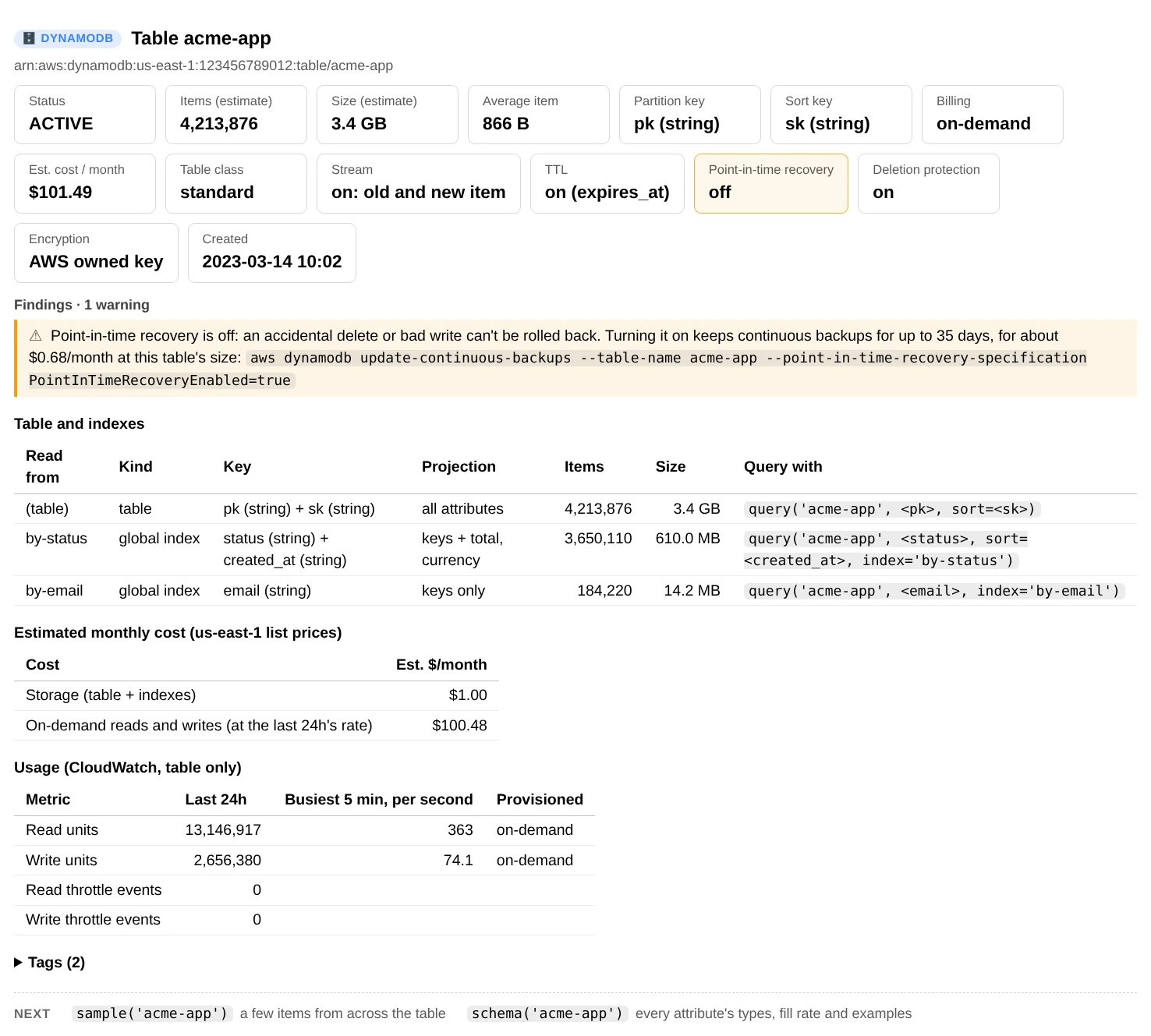
ui.table_info("acme-app"): the point-in-time recovery card is amber because the finding below is about it, and the finding ends in the command that turns it on.
In the notebook, one click on a command anywhere in a report (documents(status='FAILED'),
aws dynamodb update-table ...) or on a code block (a restore call, a lifecycle rule, a sync command) selects all of
it, ready to copy. The HTML is plain HTML and CSS, with no JavaScript, so a report still works when the notebook is
reopened. ui.help() lists every command grouped by task, with a few to start with; ui.help("summary") shows one
command's full description.
Amazon S3
Buckets and the files in them. Every bucket's size, cost and risks, what's in a folder, a look inside the files, and what you could save.
📄 analyzers/s3.py · 📖 S3 guide
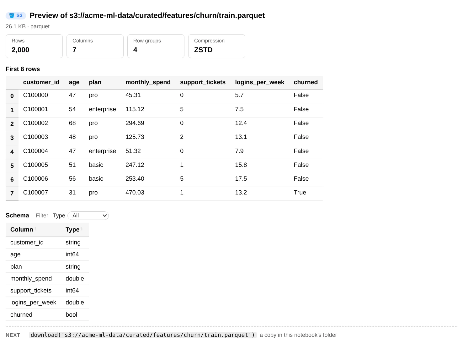
ui.preview() of a Parquet file: row, column and row-group counts, the first rows and the schema, reading only what it needs.
Quick start
Install the packages first, in a notebook cell (in a terminal, drop the %). On SageMaker the first line is already
installed, so you only need the second one, and only for the file types it lists.
%pip install boto3 pandas pyarrow      # the commands below
# optional: Excel, PDF text and pages, .zst, snappy Avro, progress bars
%pip install openpyxl xlrd pypdf pypdfium2 pillow zstandard python-snappy tqdm
# or, with pip instead of the file: all of the above and s3.py itself
%pip install "aws-analyzer[all]"
What each package is for
| Package | Needed for |
|---|---|
boto3 |
Every command (required) |
pandas |
Tables in preview (CSV, JSON, Avro, Excel, NumPy), read_df, objects_to_df, to_df(). Installs numpy for .npy / .npz |
pyarrow |
.parquet, .orc, .feather, .arrow in preview, read_df and file_details, and parquet_info |
openpyxl / xlrd |
Excel .xlsx / .xlsm and old .xls |
pypdf |
PDF text in preview, document, read_pdf, and page counts in file_details |
pypdfium2 + pillow |
PDF pages drawn as pictures, the way they print (scanned pages too), in preview, document, render_pdf. pillow also shrinks big pictures in Word files before showing them |
zstandard |
.zst files before Python 3.14 |
python-snappy |
Avro files compressed with snappy |
tqdm |
Progress bars with the time left while long commands run (ipywidgets makes them notebook widgets). Without it, a plain progress line |
IPython, used for the HTML output, comes with Jupyter. If a package is missing, the command tells you which one to install instead of failing; install it and run the cell again.
from s3 import S3View

ui = S3View()                # uses the notebook's execution role
ui.help()                    # every command, grouped by task
ui.help("summary")           # one command in full

ui.overview()                # every bucket: size, monthly cost, security warnings
ui.bucket_info("my-bucket")
ui.summary("s3://my-bucket/data/")
ui.preview("s3://my-bucket/data/part-0.parquet")
ui.what_if("s3://my-bucket/logs/", move_after=30, to="STANDARD_IA")  # preview a lifecycle rule
TIP: Anywhere a location is expected you can pass
s3://bucket/prefixorbucket/prefix. Sizes accept1024,"10MB","1.5GB"; times accept adatetime,"2024-05-01", or relative"7d","12h".
Browse like a file explorer
s3_explorer.py turns a cell into a small file explorer for S3. Folders and files are
listed on the left. Click a folder to open it, or click a file to see what's inside it on the right, drawn by the
same preview as above: a table's first rows, a PDF's pages, a Word file with its pictures, an archive's contents.

S3Explorer(): from your buckets to a Parquet file's first rows and a Word document, one click at a time.
It builds on s3.py, so put both files next to your notebook, or paste s3.py into a cell and s3_explorer.py
into the next one. Clicking needs ipywidgets, which SageMaker notebooks already have.
from s3_explorer import S3Explorer

S3Explorer()                                   # start from your buckets
S3Explorer("s3://my-bucket/data/")             # or in a folder; S3 console links work too
S3Explorer("s3://my-bucket/data/report.pdf")   # a file's folder, with the file shown
| To | Do this |
|---|---|
| Open a folder | Click it. ← → ↑ go back, forward and up, and each part of the path at the top opens that folder |
| See what's in a file | Click it. Details shows its metadata and tags, Read all a whole PDF, Word or PowerPoint file, ⬇ Download saves a copy next to your notebook, and 🔗 Link makes a download link that works for an hour |
| Go to a path | Click ✎, paste an s3:// path or an S3 console link, and press Enter |
| Narrow a long folder | Type in Filter (*.csv patterns work too). Click Name, Size or Modified to sort; sizes and dates sort biggest and newest first |
| Add up a folder | Open it and click What's in here: every file below it, with sizes, types, cost and findings (the summary report) |
Each folder is listed 1,000 entries per request and shown 100 rows at a time. In a bigger folder, Load more
lists the next 1,000, and Look up asks S3 for the names that start with what you typed in the filter. Files in
GLACIER or DEEP_ARCHIVE are marked ❄, and opening one shows the command that restores it. Like s3.py, it only
reads: browsing needs s3:ListAllMyBuckets and s3:ListBucket, and opening files s3:GetObject.
Options, and using it from code
from s3 import S3Analyzer
from s3_explorer import S3Explorer, S3Navigator

S3Explorer("s3://my-bucket/", profile="dev")          # another AWS profile (or region=)
S3Explorer(core=S3Analyzer(region="eu-west-1"))       # an S3Analyzer or S3View you already have
S3Explorer(height=720, page_size=200)                 # taller panes, more rows before "Show more"

x = S3Explorer("s3://my-bucket/")
x.open("s3://my-bucket/raw/"); x.back(); x.up(); x.refresh()   # the toolbar, from code
x.ui.summary(x.location)                              # any S3View report about where you are, in its own cell

nav = S3Navigator()                                   # the same navigation as data, with no UI
folder = nav.open("s3://my-bucket/data/")             # Folder: entries, more, error
nav.more(), nav.back(), nav.up(), nav.lookup("2024-")
Outside Jupyter, without ipywidgets, or with mode="text", each folder prints as a table and open(...) moves
around. The pure functions work on their own: parse_location (s3:// paths, bucket/key, console links and object
URLs), breadcrumbs, parent_uri, sort_entries (folders first, part-2 before part-10), filter_entries and
folder_stats.
Commands (S3View)
Grouped the way ui.help() lists them.
Buckets
| Command | Shows |
|---|---|
buckets() |
All buckets with region, creation date, age |
overview(match=None) |
Every bucket in one table: objects, size, estimated monthly cost, versioning, encryption, public access, lifecycle rules, and a list of warnings. match="sagemaker-*" checks only matching names |
bucket_info(bucket) |
Versioning, encryption, public access (bucket and account level), bucket policy and lifecycle rules in plain English, ownership, object lock, replication, logging, inventory, tags, plus CloudWatch object count, size and estimated monthly cost per storage type (instant, even for billion-object buckets), and flagged risks |
policy(bucket) |
The bucket policy in plain English (who can do what, on which files, under which conditions), its risks (public access, other accounts, no HTTPS requirement) and the raw JSON |
Explore a folder
| Command | Shows |
|---|---|
ls(uri, details=False) |
One level of folders and files, like aws s3 ls. details=True adds what's inside each file: a PDF's pages, a table's rows and columns, a picture's size |
tree(uri, depth=2, files=10) |
Folder tree with count, size and share at every level, and the files in each folder (the first files by name, then one "… N more files" row; files=0 for folders only) |
summary(uri) |
Dashboard: totals, estimated monthly cost, folder breakdown, file types, storage classes, size and age histograms, largest objects, and findings (small-file problem, archived objects, cold data in STANDARD and what moving it would save, files under 128 KB billed as 128 KB, empty files) |
find(uri, pattern=, regex=, extensions=, min_size=, max_size=, modified_after=, modified_before=, storage_classes=) |
Search by glob, regex, extension, size, date or storage class, e.g. find(uri, pattern="*.csv", min_size="10MB", modified_after="7d") |
file_details(uri, pattern=, extensions=, limit=200, max_read="1GB") |
What's inside each file, a table per kind (see what it reports): a PDF's pages, title, author and whether it has text, a Word file's words, a deck's slides, each Excel sheet's size, a table's rows and column names, a picture's size, a video's length, an archive's files. Findings: scanned PDFs that need OCR, password-protected files, files that aren't what their name says, table files in one folder with different columns. Reads only the parts each format needs |
largest(uri) / newest(uri) / oldest(uri) |
The top-N objects under a prefix: the biggest, the newest or the oldest |
compare(uri_a, uri_b) |
Diff two prefixes: identical / different / only in A / only in B (to verify a copy or sync) |
Cut cost
| Command | Shows |
|---|---|
duplicates(uri, method="hash", min_size=1, max_read="10GB") |
Identical files, the space and monthly cost of their copies, which copy to keep, and folders that hold nothing but copies (e.g. a backfill of files that exist elsewhere), plus the call that gets the list as a DataFrame. Files are matched by size and ETag, and where same-size files have different ETags (copies uploaded in parts of another size, or encrypted with SSE-KMS), by the SHA-256 of their content: the first 64 KB first, the whole file only where those match, reading at most max_read. method="etag" reads nothing; method="strict" hashes every file that shares its size |
what_if(uri, move_after=, to=, delete_after=) |
Preview a lifecycle rule before adding it: how many files it would move or delete today, cost before and after, one-time cost and payback time, plus the rule's JSON. move_after={30: "STANDARD_IA", 180: "GLACIER"} for several moves |
uploads(uri) |
Incomplete multipart uploads (billed but invisible in normal listings) and what they cost |
Versions and deleted files
| Command | Shows |
|---|---|
versions(uri) |
Current vs noncurrent versions, delete markers, what the old versions cost per month, keys holding the most old-version data |
history(uri) |
Version history of one object |
deleted(uri, deleted_after=None) |
Deleted files you can still bring back in a versioned bucket (most recent first), their size, the old versions kept, and the call that restores one. Read-only: it never restores anything itself |
Open a file
| Command | Shows |
|---|---|
head(uri) |
All object metadata, user metadata and tags |
preview(uri, n=20) |
Looks inside a file (see file types): tables as a DataFrame with their schema, the files in an archive, tensors, notebook cells, pretty JSON, text, images, an audio / video player, a PDF's first pages as they look (scans too), a Word file with its pictures in place, or a hex dump. Only downloads what it needs. |
document(uri, pages=None, pictures=None) |
A PDF, Word .docx or PowerPoint .pptx as it reads: a Word file with its headings, lists, tables and pictures in place, a PDF or deck page by page or slide by slide. PDF pages with no text (scans) are drawn as pictures; pictures=True draws every page. PDFs need pypdf, and pypdfium2 + pillow to draw pages |
download(uri, path=None) |
Downloads a file, or a whole folder with its sub-folders, with a progress bar, and says where it went. Files already there with the same size and time are skipped, so running it again resumes. GLACIER files are listed as needing a restore, and it refuses when the disk hasn't room. For a table file it shows the pandas call that opens it |
download_zip(uri, path=None, max_size="100MB", max_files=10_000, dry_run=False) |
A file or folder as one .zip on the notebook's disk, but first a check of whether this notebook can make it: the files fit the size limit (100 MB by default) and file count, the disk has room, memory, and the role can read them (one 1-byte read). If a check fails nothing is downloaded, and the report says what to change (e.g. the max_size= that would fit). dry_run=True only runs the checks. GLACIER files are left out and listed; parquet, gz and images are stored as they are, the rest compressed |
link(uri) |
Clickable presigned download link |
Reference
Getting the data (S3Analyzer): the same answers as Python data, for pandas and your own code
ui.core is the S3Analyzer. Every UI command has a data method on it, and there are a few more:
s3 = ui.core                                        # or S3Analyzer(region="us-east-1", profile="dev")

summary = s3.summarize("s3://my-bucket/data/")      # PrefixSummary dataclass
summary.by_extension["parquet"].size                # bytes

files = s3.find("s3://my-bucket/data/", extensions=["csv"], modified_after="7d")
df = objects_to_df(files)                           # key, size, last_modified, storage_class, ...

df = s3.read_df("s3://my-bucket/data/big.parquet", nrows=1000, columns=["id", "ts"])
df = s3.read_df("s3://my-bucket/reports/q1.xlsx", sheet_name="Summary")
df = s3.read_df("s3://my-bucket/spark/part-00000", fmt="parquet")   # no extension: say what it is
s3.parquet_info("s3://my-bucket/data/big.parquet")  # rows, row groups, schema (reads only the footer)
s3.list_archive("s3://my-bucket/job/output/model.tar.gz").entries   # files inside, without extracting
details = s3.file_details("s3://my-bucket/docs/", extensions="pdf")   # FileDetailsReport: .files, bytes_read
details.to_df()                                     # one row per file: format, size, summary, pages, title, rows, ...
s3.describe_objects(s3.find("s3://my-bucket/", min_size="1GB"))     # the same, for files you picked
s3.read_avro("s3://my-bucket/events.avro", n=100), s3.read_npy(uri, nrows=10), s3.safetensors_info(uri)
doc = s3.read_document("s3://my-bucket/docs/policy.pdf")   # also .docx / .pptx: doc.text, doc.parts, doc.title
s3.read_pdf(uri, pages=[1, 2]), s3.read_docx(uri).headings, s3.read_pptx(uri).notes
pages = s3.render_pdf(uri, pages=[1, 2])            # [Picture]: each one shows itself in a notebook; .data is PNG / JPEG
s3.read_docx(uri, pictures=True).pictures           # the pictures in a Word file, in reading order
s3.read_lines("s3://my-bucket/logs/app.log.gz", 50)
s3.read_json(...), s3.read_jsonl(..., n=100), s3.read_text(...), s3.read_bytes(uri, 0, 1023)
with s3.open("s3://my-bucket/data/x.csv.gz") as f: ...   # streaming, decompressed

for obj in s3.iter_objects("s3://my-bucket/"):      # stream a listing without holding it in memory
    ...

reports = s3.bucket_reports(match="sagemaker-*")    # BucketConfig + CloudWatch size per bucket
explain_policy(s3.bucket_policy("my-bucket"), s3.account_id())   # [PolicyStatement], plain English
impact = s3.simulate_lifecycle("s3://my-bucket/logs/", move_after=30, to="STANDARD_IA")
impact.monthly_savings, impact.rule()               # USD per month, the rule as a dict
s3.deleted_files("s3://my-bucket/data/", deleted_after="7d").files   # [DeletedObject]
dupes = s3.find_duplicates("s3://my-bucket/data/")  # DuplicateReport: groups, copies, reclaimable, monthly_cost
dupes.to_df()                                       # one row per file: group, role ('keep' / 'copy'), key, sha256, ...
s3.download_folder("s3://my-bucket/data/", "data")  # FolderDownload; s3.download(uri, path) for one file
plan = s3.plan_zip("s3://my-bucket/data/")          # ZipPlan: files, size, disk / memory free, can_download
s3.download_zip("s3://my-bucket/data/", max_size="1GB").plan.path   # ZipDownload; nothing written if a check fails
The aggregation functions are pure (no AWS calls), so they also work on your own lists of ObjectInfo,
for example rows loaded from an S3 Inventory report: summarize_objects, build_folder_tree,
make_filter, find_duplicate_groups, compare_objects, simulate_lifecycle_objects, summary_findings,
bucket_findings, explain_policy, policy_findings, object_monthly_cost, cloudwatch_cost, the duplicate
finder's steps (files_to_hash says which files need reading, group_duplicates groups them given the hashes you
have, then duplicate_folders and duplicate_findings), zip_checks and zip_findings (on a ZipPlan), and the
file parsers parse_docx (pictures=True for its pictures), parse_pptx, parse_pdf, parse_avro, and
render_pdf_pages, which draws a PDF's pages from a local file or bytes. describe_file("local.pdf") (or a binary file
object and its name) says what's inside a file the way file_details does, and file_details_findings works on a
FileDetailsReport.
File types: what preview and read_df can open
preview and read_df pick the reader from the file name, and from the first bytes when the name has
no extension or the wrong one (Spark's part-00000, a Firehose object, a .gz that isn't gzipped).
| Kind | Extensions | preview shows |
read_df |
|---|---|---|---|
| Delimited text | .csv .tsv .psv |
first rows | ✓ |
| JSON | .json .jsonl .ndjson |
table of records, or pretty JSON | ✓ |
| Columnar | .parquet .orc .feather .arrow |
first rows, schema, row count (reads only what it needs) | ✓ |
| Avro | .avro |
first rows, schema, codec (built-in reader; snappy needs python-snappy) |
✓ |
| Excel | .xlsx .xlsm .xls |
sheet names, first rows (needs openpyxl; .xls needs xlrd) |
✓ sheet_name= |
| NumPy | .npy .npz |
shape, dtype, first rows / the arrays inside | ✓ .npy up to 2-D |
| Archives | .zip .tar .tar.gz .tgz |
the files inside, e.g. a SageMaker model.tar.gz |
|
| Models | .safetensors .pt .pth .ckpt .pkl .joblib |
tensors, shapes, parameter count / files inside; pickles are never loaded | |
| Notebooks | .ipynb |
kernel and cells | |
| Images, audio, video | .png .jpg .gif .webp / .wav .mp3 .flac / .mp4 .webm .mov |
the image / a player | |
.pdf |
the first 3 pages as they look, scanned pages too (needs pypdfium2 + pillow), page count, title and first page's text (needs pypdf); without either, a link |
||
| Word | .docx .docm .dotx |
the first paragraphs laid out with their headings, lists, tables and pictures in place; word count (no package needed) | |
| PowerPoint | .pptx .pptm .ppsx |
every slide's title and text, speaker notes (no package needed) | |
| Old Office | .doc .ppt .msg |
recognised, with how to convert them (the old binary format can't be read) | |
| Text | .txt .log .md .yaml .xml .sql .py and more |
first lines |
Any of them can also be compressed: .gz, .bz2, .xz, or .zst (Python 3.14+, or pip install zstandard).
Packages in the table are optional; without them preview says what to install.
File details: what file_details and ls(details=True) report for each kind of file
Each file's format comes from its name and is checked against its first bytes, so a file with no extension is still
described and one with the wrong extension is flagged ("report.pdf is text, not a PDF"). Counts marked ≈ are
estimates from the start of the file, and + marks a lower bound.
| Kind | Extensions | Reports | Reads |
|---|---|---|---|
.pdf |
pages, whether the first 3 pages have text (none = probably scanned), page size (A4, Letter, …), title, author, the app that made it, creation date, PDF version, whether it needs a password | the page tree and first 3 pages (needs pypdf) |
|
| Word | .docx .docm .dotx |
words, pages (as Word last saved them), headings, tables, pictures, title, author, last saved | the document's text |
| PowerPoint | .pptx .pptm .ppsx |
slides, words, slides with speaker notes, tables, pictures, title, author | the slides' text |
| Excel | .xlsx .xlsm |
each sheet's name and rows × columns, title, author | the size saved at the top of each sheet |
| Parquet | .parquet |
rows, column names, row groups, compression, the program that wrote it | the footer (needs pyarrow) |
| ORC, Feather | .orc .feather .arrow |
rows, column names, compression, stripes / record batches | the metadata (needs pyarrow) |
| Avro | .avro |
rows, column names, codec | block headers, in files up to 64 MB |
| CSV, JSON lines | .csv .tsv .psv .jsonl .ndjson |
column names, rows: exact up to 256 KB, then ≈ estimated, or + when compressed |
the first 256 KB |
| JSON | .json |
records and their keys, or an object's keys | up to 16 MB |
| Pictures | .png .jpg .gif .bmp .webp, TIFF |
format, width × height | the first 64 KB |
| Audio, video | .wav .flac .mp4 .mov .m4a |
length; sample rate and channels; width × height | the header / the MP4 moov box |
| Archives | .zip .tar .tar.gz .tgz |
files inside, unpacked size | the zip index / tar headers |
| Models, arrays | .safetensors .npy .npz .pt .pth .pkl |
tensors, parameters, dtypes / shape / arrays / files inside; pickles are never loaded | headers only |
| Notebooks | .ipynb |
cells, code cells, outputs, kernel | up to 50 MB |
| Text | .txt .log .md and more |
lines | the first 256 KB |
Cost estimates: storage only, at us-east-1 list prices, or yours
Costs are storage only (no requests, retrievals or data transfer), at us-east-1 list prices for the first
50 TB (S3_PRICES). They follow S3's billing rules: STANDARD_IA, ONEZONE_IA and GLACIER_IR bill at least
128 KB per object, and GLACIER / DEEP_ARCHIVE add 40 KB of index data per object. Listings don't say which
Intelligent-Tiering tier an object is in, so it's priced at the frequent-access rate; CloudWatch does, so
bucket_info and overview price each tier. For another region, pass your prices:
ui = S3View(S3Analyzer(prices={"STANDARD": 0.025, "STANDARD_IA": 0.0138}))
Large buckets: how long each command takes on millions of objects, and what to run first
summary,tree,find,duplicatesandcomparelist every key under the prefix (1,000 per request), so expect about 1 to 3 minutes per million objects. A progress bar shows while they run. Passlimit=to sample.duplicatesalso downloads files that share a size but not an ETag: 64 KB of each, then whole files only where those match, 16 at a time, biggest possible saving first, and it stops atmax_read(10 GB by default). It says how much it read. That download is free inside the bucket's region; from outside AWS it's billed as data transfer.method="etag"reads nothing.download_zipcounts at mostmax_fileskeys (10,000 by default) before it decides, so it answers quickly even on a huge folder, and it only downloads once every check passes.what_iflists every key too;deletedandversionslist every version.bucket_inforeads the bucket's size from CloudWatch without listing anything. Use it first on huge buckets.overviewmakes about 15 read calls per bucket, 8 buckets at a time, and lists no keys.file_detailslooks inside the first 200 files (limit=), 8 at a time, in 256 KB ranged requests, reading only what each format needs (a PDF's page tree, a parquet footer, a picture's header), at most 128 MB of one file, and stops atmax_read(1 GB by default). It says how much it read.lsonly lists one level, so it's fast anywhere.ls(details=True)also reads a little of each file listed.
IAM permissions: read-only, and what each one is for
Read-only. Grant what you need:
| Permission | For |
|---|---|
s3:ListAllMyBuckets, s3:GetBucketLocation |
The list of buckets (also the explorer's first page), and each bucket's region |
s3:ListBucket, s3:ListBucketVersions |
Listing files (also in the explorer), their old versions and delete markers |
s3:ListBucketMultipartUploads, s3:ListMultipartUploadParts |
Incomplete multipart uploads |
s3:GetObject |
Reading files: preview, document, file_details, ls(details=True), duplicates, download / download_zip |
s3:GetObjectTagging |
Object tags |
The s3:GetBucket* / s3:GetLifecycleConfiguration / s3:GetReplicationConfiguration / s3:GetEncryptionConfiguration / s3:GetInventoryConfiguration family |
The settings in bucket_info, including s3:GetBucketPolicy for policy |
s3:GetAccountPublicAccessBlock |
The account-level public access setting |
cloudwatch:ListMetrics, cloudwatch:GetMetricData |
Bucket sizes |
Anything you can't read shows up as a note instead of an error. The S3 guide has a ready-made IAM policy that covers every command.
Amazon DynamoDB
Tables and the items in them. Every table's keys, size, billing and cost, the items as plain tables, and what they hold.
📄 analyzers/dynamodb.py · 📖 DynamoDB guide
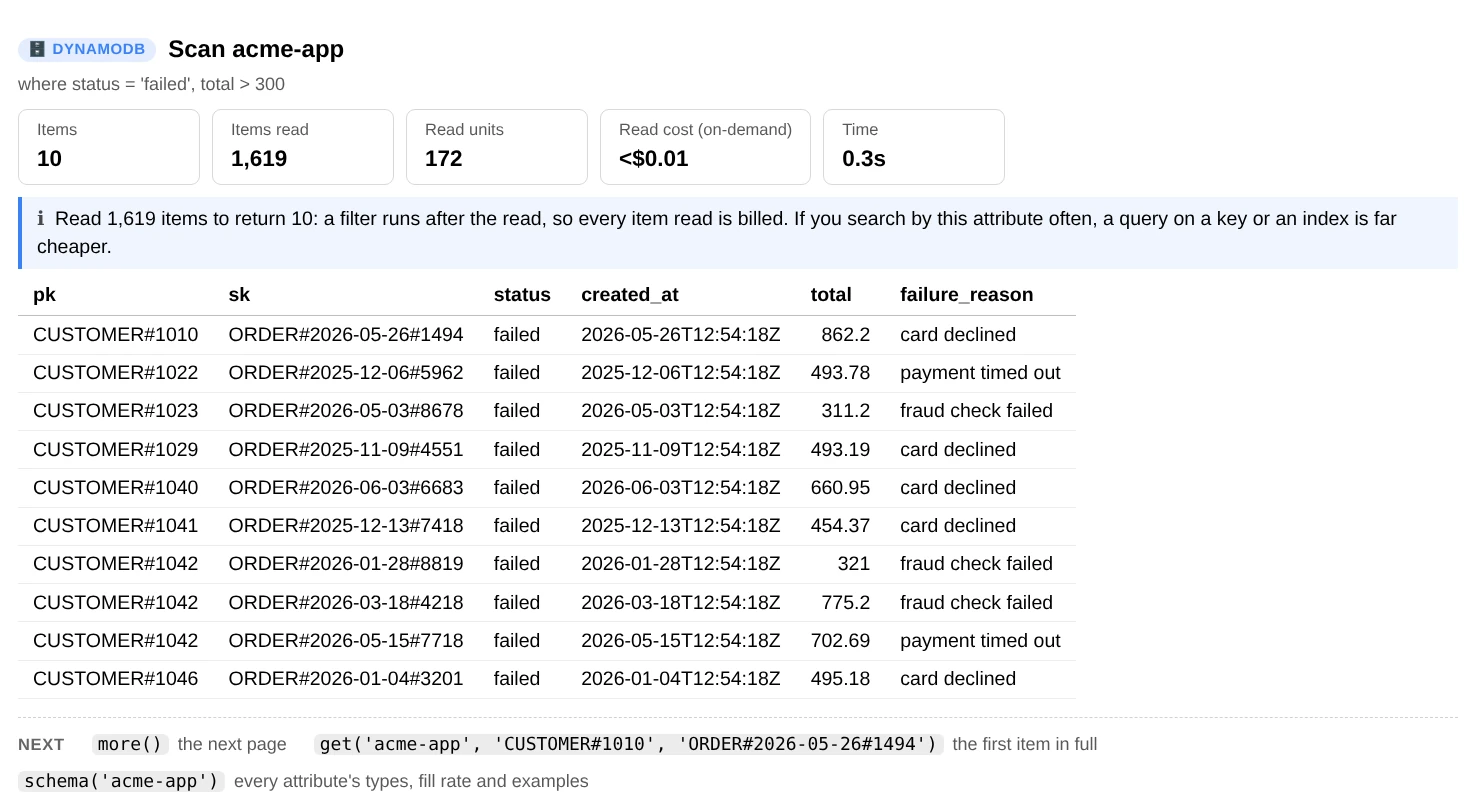
ui.scan() with a where= filter: ten failed orders over 300, found by reading 1,619 items, the read units that took, and why a query would be cheaper.
Quick start
Install the packages first, in a notebook cell (in a terminal, drop the %). On SageMaker both are already
installed.
%pip install boto3    # every command (required)
%pip install pandas   # optional: DataFrames (page.to_df(), profile.to_df(), items_to_df)
Every DynamoDBView command works with boto3 alone; IPython, used for the HTML output, comes with Jupyter.
from dynamodb import DynamoDBView

ui = DynamoDBView()          # uses the notebook's execution role and region
ui.help()                    # every command, grouped by task
ui.help("scan")              # one command in full

ui.tables()                  # every table in the region: key, items, size, est. cost, warnings
ui.table_info("orders")      # indexes and how to query each, capacity, usage, backups, risks
ui.scan("orders")            # the first 20 items as a table...
ui.more()                    # ...and the next 20
ui.schema("orders")          # what the items look like
ui.get("orders", "USER#42", "ORDER#0017")
ui.query("orders", "USER#42", sort=("begins_with", "ORDER#"))
NOTE: Tables are regional:
DynamoDBView(DynamoDBAnalyzer(region="eu-west-1"))looks at another region. Items are shown and returned as plain Python, not DynamoDB JSON: numbers areint/float, sets are sets, binary isbytes. Nothing in the file writes to a table.
Commands (DynamoDBView)
Grouped the way ui.help() lists them.
Tables
| Command | Shows |
|---|---|
tables(match=None) |
Every table in the region in one table: key, item count, size, billing mode, indexes, estimated monthly cost (including on-demand requests at the last 24 hours' rate) and a list of warnings. match="prod-*" checks only matching names |
table_info(table) |
Keys and types, every index with its projection and the query(...) call that reads it, billing and capacity, CloudWatch usage over the last 24 hours (consumed units, busiest 5 minutes, throttling), TTL, stream, point-in-time recovery, deletion protection, encryption, tags, estimated monthly cost, and flagged risks, each with what to do about it: no point-in-time recovery (with its cost and the command that turns it on), throttling, capacity near its limit, or capacity far above what's used (with what less capacity or on-demand would cost) |
Look at items
| Command | Shows |
|---|---|
sample(table, n=20) |
About n items spread across the whole key space. scan shows the start of the table, which can all be one partition key; this reads a few items from many slices of it |
scan(table, n=20, where=, index=, attributes=) |
Items from the start of the table (or an index) as a table: key attributes first, then the others by how many items have them, nested maps as address.city columns. Shows how many items were read to find them and the read units used |
query(table, partition, sort=None, index=, where=, descending=) |
Items sharing one partition key, in sort-key order, on the table or an index |
get(table, *key) |
One item with every nested map and list expanded, the type of each attribute, its size and read / write cost. as_json=True adds a JSON copy |
sql(statement, *params) |
A PartiQL statement, e.g. sql('SELECT * FROM "orders" WHERE pk = ?', "USER#42") |
more() |
The next page of the last scan, query or sql |
Understand the data
| Command | Shows |
|---|---|
schema(table, n=1000) |
Every attribute and map field: type (or mix of types), share of items that have it, distinct values, examples, range. Key patterns such as USER#<number> and ORDER#<date>, which show the entity types of a single-table design. Item sizes, the largest items, and findings: mixed types, empty strings, items near the 400 KB limit, attribute names built from data |
value_counts(table, attribute) |
How often each value occurs, with the size of those items. On the partition key this is each item collection's size, so hot partitions stand out |
largest(table, n=10) |
The biggest items by DynamoDB's sizing rules, and what reading each costs |
count(table, where=None) |
Exact count (a full scan), next to DynamoDB's own estimate |
Filters
where= works on scan, query, sample, schema, value_counts, largest and count. It takes a dict, and
every condition must match:
where= |
Means |
|---|---|
{"status": "failed"} |
status = 'failed' |
{"total": (">", 100)} |
also "=", "!=", "<", "<=", ">=" |
{"total": ("between", 10, 100)} |
both ends included |
{"sk": ("begins_with", "ORDER#")} |
|
{"tags": ("contains", "promo")} |
a substring, or a member of a set or list |
{"status": ("in", ["paid", "shipped"])} |
|
{"deleted_at": ("not_exists",)} |
also ("exists",), and ("type", "N") to check the stored type |
{"address.city": "Pune"} |
dots reach into maps |
For OR and NOT, pass a boto3 condition instead: where=Attr("a").eq(1) | Attr("b").exists(). The sort= argument
of query takes a value or one of the same tuples (=, <, <=, >, >=, between, begins_with). Key values
are converted to the key's type, so "42" works for a number key.
Reference
Getting the data (DynamoDBAnalyzer): items as plain dicts and DataFrames, for pandas and your own code
ui.core is the DynamoDBAnalyzer. Every UI command has a data method on it:
ddb = ui.core                                       # or DynamoDBAnalyzer(region="eu-west-1", profile="dev")

page = ddb.scan("orders", n=5000, where={"status": "failed"})   # ItemPage
page.items                                          # list of plain dicts
df = page.to_df()                                   # DataFrame: keys first, nested maps as 'address.city'
page.stats                                          # items read, items returned, read units, seconds
more = ddb.scan("orders", n=5000, where={"status": "failed"}, start_key=page.last_key)

ddb.query("orders", "USER#42", sort=("between", "ORDER#2024-01", "ORDER#2024-12"), descending=True)
ddb.query("orders", "failed", index="by-status").to_df()
ddb.sample("orders", 500).items                     # spread over the key space
ddb.get("orders", "USER#42", "ORDER#0017")          # dict, or None
ddb.sql('SELECT * FROM "orders" WHERE pk = ?', "USER#42").items

profile = ddb.profile("orders", 2000)               # TableProfile (what schema() shows)
profile.attributes["total"].types                   # Counter({'N': 1990, 'S': 10})
profile.to_df()                                     # one row per attribute

ddb.value_counts("orders", "status").counts         # {'paid': Stat(count=..., size=...), ...}
ddb.count("orders", where={"status": "failed"}).matched
ddb.describe("orders")                              # TableInfo: keys, indexes, capacity, TTL, backups, tags
ddb.table_metrics("orders", hours=24)               # consumed units, busiest period, throttle events
ddb.table_reports(match="prod-*")                   # [TableReport]: describe() + usage for every table

for item in ddb.iter_items("orders", limit=None):   # stream a full scan without holding it in memory
    ...
The analysis functions are pure (no AWS calls), so they also work on items you already have, for example a
DynamoDB export to S3: from_dynamo_item, to_dynamo, items_to_df, flatten_item, profile_items,
count_values, item_size, key_pattern, build_filter, table_findings, profile_findings,
table_monthly_cost, capacity_cost, request_cost.
rows = S3Analyzer().read_jsonl("s3://my-bucket/AWSDynamoDB/01234-abcd/data/part.json.gz")   # from s3.py
profile_items([from_dynamo_item(row["Item"]) for row in rows], keys=["pk", "sk"])
Large tables and cost: what scans read and bill, where they stop, and the prices used
- DynamoDB bills every item a scan reads, and a scan competes with your application for the table's
capacity. So the commands that scan stop early by default:
value_countsandlargestread the first 10,000 items (limit=Nonereads everything),schemaprofiles about 1,000, andui.scanwith a filter reads at most 100,000 items per page (scan_limit=). countalways reads the whole table:Select=COUNTreturns no items but still reads, and bills, every one. For an instant estimate,tables()andtable_info()show DynamoDB's own item count and size, which it refreshes about every 6 hours.- Every report shows the read units it used and, where it matters, what they cost on-demand.
- Costs are estimates at us-east-1 list prices for the standard table class, before the free tier
(
DYNAMODB_PRICES): storage, provisioned capacity and point-in-time recovery per month, and on-demand reads and writes per million. For another region, pass your prices:DynamoDBAnalyzer(prices={"storage": 0.285, "read_request": 0.1425}).
IAM permissions: read-only, and what each one is for
Read-only. Grant what you need:
| Permission | For |
|---|---|
dynamodb:ListTables |
The list of tables |
dynamodb:DescribeTable, dynamodb:DescribeTimeToLive, dynamodb:DescribeContinuousBackups, dynamodb:ListTagsOfResource |
A table's keys, indexes and settings |
dynamodb:Scan, dynamodb:Query, dynamodb:GetItem |
Reading items |
dynamodb:PartiQLSelect |
sql |
cloudwatch:GetMetricData |
Usage |
Reading an index needs the permission on its ARN too (arn:aws:dynamodb:<region>:<account>:table/orders/index/*),
and a table encrypted with a customer managed KMS key needs kms:Decrypt. Anything you can't read shows up as a
note instead of an error. The DynamoDB guide
has a ready-made IAM policy that covers every command.
Amazon Bedrock Knowledge Bases
Knowledge bases, what they retrieve, and the answers built on them. Settings and sync health, search with highlighted passages, answers with citations, and retrieval measured on your own questions.
📄 analyzers/bedrock_kb.py · 📖 Knowledge Bases guide
![ask(): an answer about refund times with a [1] and a [2] marker, 77% grounded because its last sentence cites nothing, cards for sources used, model, estimated tokens, cost and time, and the two cited passages from refund-policy.pdf](https://pypi-camo.freetls.fastly.net/9fbf3754c53e4d224859f5ae84905b4f6fe37835/68747470733a2f2f7261772e67697468756275736572636f6e74656e742e636f6d2f75746b61727368353032362f6177732d616e616c797a65722f6d61696e2f646f63732f696d616765732f626564726f636b2d61736b2d6c696768742e77656270)
ui.ask("How long do refunds take?"): the answer with its [1] [2] citations, 77% grounded because its last sentence cites nothing, and the passages behind it.
Quick start
Install the packages first, in a notebook cell (in a terminal, drop the %). On SageMaker both are already
installed.
%pip install boto3    # every command (required)
%pip install pandas   # optional: DataFrames (r.to_df(), a.to_df(), report.to_df())
Every BedrockKBView command works with boto3 alone; IPython, used for the HTML output, comes with Jupyter.
Answers are generated through Bedrock itself (RetrieveAndGenerate or Converse), so no model SDK is needed and any
Bedrock model you have access to works.
from bedrock_kb import BedrockKBView

ui = BedrockKBView()               # uses the notebook's execution role and region
ui.help()                          # every command, grouped by task
ui.help("ask")                     # one command in full

ui.kbs()                           # every knowledge base: status, store, last sync, warnings
ui.use("support-docs")             # later commands use this one (a name, ID or ARN)
ui.kb_info()                       # settings in plain English, syncs, findings, idle cost
ui.search("how do refunds work?")  # ranked passages, with the question's words highlighted
ui.chunk(2)                        # the full text and metadata of result #2
ui.ask("How long do refunds take?")      # an answer with [1][2] citations and its sources
ui.follow_up("And for digital goods?")   # same conversation
NOTE: Knowledge bases are regional:
BedrockKBView(BedrockKBAnalyzer(region="us-west-2"))looks at another region. Commands takekb=(a name in any case, the 10-character ID, or the ARN); without it they use the one set byuse()orBedrockKBView(kb=...), else the only knowledge base in the region, else they list the ones there and say how to pick. Nothing in the file changes a knowledge base: where a sync is needed, it shows theaws bedrock-agent start-ingestion-job ...command and the boto3 call instead of running them.
Commands (BedrockKBView)
Grouped the way ui.help() lists them.
Knowledge bases
| Command | Shows |
|---|---|
kbs() |
Every knowledge base in the region: status, type, vector store, embedding model, data sources, documents read by the last sync, last sync, estimated idle cost and warnings |
use(kb) |
Sets the knowledge base that later commands use when you don't pass kb=: a name in any case, the 10-character ID, or the ARN |
kb_info(kb=None) |
Cards (status, vector store, embedding model and dimensions, data sources, last sync, idle cost), findings, every setting in plain English (vector store, each data source's location, chunking, parsing and deletion policy), recent syncs, tags, and what to try next |
What's indexed
| Command | Shows |
|---|---|
syncs(kb=None, data_source=None, n=10) |
Sync history: when, how long, status, scanned / new / modified / deleted / failed counts, why syncs failed, and the command to sync again |
documents(kb=None, data_source=None, status=None, n=50) |
Documents by status (indexed, failed, pending ...), the ones that aren't indexed with Bedrock's reason, and the sync command. status="INDEXED" or "FAILED" lists only those |
unsynced(kb=None, data_source=None) |
S3 files added or changed since each data source's last successful sync, and the command to sync them |
Search and answer
| Command | Shows |
|---|---|
search(question, n=5, kb=, where=, search_type=, rerank=) |
Ranked passages: a score bar relative to the top result, file and page, the best part of the text with the question's words highlighted, and the passage's metadata. Findings: nothing found, one file answering everything, duplicate passages, very short chunks, and codes in the question that no passage contains (try search_type="HYBRID"). Time and estimated cost |
chunk(rank) |
The full text, metadata and IDs of result #rank from the last search or ask, and the S3View().preview("s3://...") call that opens its file |
ask(question, kb=, n=5, where=, model=, engine="kb", prompt=, temperature=, max_tokens=) |
The answer with [1][2] citation markers, cards (grounded share, sources used, model, tokens, cost, time), the sources table and findings (not grounded, mostly uncited, Bedrock's "unable to assist" reply, a guardrail, cut off at max_tokens) |
follow_up(question) |
The next question in the same RetrieveAndGenerate session (or Converse conversation). If the session has expired, starts a new one and says so |
models(match=None) |
The text models you can use for ask() here: the ID to pass as model=, provider, on demand or through an inference profile, and $ per 1M tokens in and out |
Measure retrieval
| Command | Shows |
|---|---|
compare(question, kb=, n=(5, 10), search_types=("SEMANTIC", "HYBRID"), where=) |
One row per passage and one column per setting with its rank there, how much each pair of settings overlaps, and what each found that the others missed |
evaluate(cases, kb=, n=5, search_type=) |
Retrieval hit rate @n and MRR on test questions, where each expected source ranked (or "missed") and what came up first instead, with the usual fixes |
Two ways to generate answers
engine="kb" (default) |
engine="converse" |
|
|---|---|---|
| How | Bedrock's managed RetrieveAndGenerate: Bedrock retrieves, prompts the model and returns the citations | Retrieves, then calls the model through Bedrock Converse with the passages numbered as sources. Any Bedrock model |
| Tokens and cost | Estimated from characters, and labelled as estimates: RetrieveAndGenerate doesn't report token counts | Exact counts and cost |
| Your own prompt | A custom prompt= must contain $search_results$ |
A prompt= template with {sources} and {question} (see bedrock_kb.DEFAULT_PROMPT) |
| Follow-ups | follow_up() keeps Bedrock's session |
follow_up() continues the conversation |
With engine="converse", the sources are sent as data, never as instructions, and the model is told to cite them as
[n] and to say when they don't hold the answer.
model= takes a model ID or ARN, an inference profile ID, or a short name: "opus", "sonnet", "haiku",
"claude-opus-5", "nova-pro". The default is Claude Opus 5 (bedrock_kb.DEFAULT_MODEL), through the region's
inference profile when it needs one; BedrockKBAnalyzer(default_model="sonnet") changes it.
Filters (where=)
where= filters on the documents' own metadata, which comes from a <file>.metadata.json next to each file (for
example refund-policy.pdf.metadata.json holding {"metadataAttributes": {"team": "billing", "year": 2024}}). It
works on search, ask, compare and evaluate, uses the same vocabulary as the DynamoDB analyzer, and every
condition must match:
where= |
Means |
|---|---|
{"team": "billing"} |
team = 'billing' |
{"team": ["billing", "support"]} |
one of these values |
{"year": (">=", 2024)} |
also "=", "!=", ">", "<", "<=" |
{"year": ("between", 2020, 2024)} |
both ends included |
{"region": ("in", ["eu", "uk"])} |
also ("not_in", [...]) |
{"doc_id": ("begins_with", "POL-")} |
text starting with this |
{"title": ("contains", "refund")} |
text containing this, or a list with an element containing it |
{"tags": ("list_contains", "gdpr")} |
a list attribute holding exactly this element |
Values are typed: 2024 and "2024" differ. For OR, pass a Bedrock RetrievalFilter instead, e.g.
where={"orAll": [{"equals": {"key": "team", "value": "a"}}, {"equals": {"key": "team", "value": "b"}}]}; it is
sent unchanged.
Reference
Getting the data (BedrockKBAnalyzer): passages, answers and evaluations as Python objects
ui.core is the BedrockKBAnalyzer. Every UI command has a data method on it, and its methods take the knowledge
base first:
kb = ui.core                                        # or BedrockKBAnalyzer(region="us-west-2", profile="dev")

info = kb.describe("support-docs")                  # KnowledgeBaseInfo: settings, data sources, last syncs, tags
info.data_sources[0].chunking                       # the chunkingConfiguration AWS returned
kb.list_knowledge_bases()                           # [KnowledgeBaseInfo], described in parallel
kb.ingestion_jobs("support-docs", n=20)             # [IngestionJob], newest first, with failure reasons
docs, summary = kb.documents("support-docs", status="FAILED")   # [KBDocument], DocumentSummary
kb.unsynced("support-docs")                         # [SyncFreshness]: changed S3 files per data source

r = kb.retrieve("support-docs", "refund window", n=10, where={"team": "billing"})   # Retrieval
r.passages[0].text, r.passages[0].source, r.passages[0].metadata
df = r.to_df()                                      # one row per passage

a = kb.ask("support-docs", "How long do refunds take?")          # Answer (RetrieveAndGenerate)
a.text, a.citations, a.sources, a.grounded_share
a = kb.generate("refund window?", r.passages, model="opus", prompt=MY_TEMPLATE)   # Converse on your passages
a = kb.generate("refund window?", ["my own chunk", "another chunk"])             # ...or on plain strings
a.input_tokens, a.output_tokens                     # exact, from Converse

kb.compare("support-docs", "refund window for EU orders").overlap   # SearchComparison
report = kb.evaluate("support-docs", [("refund window?", "refund-policy.pdf")])
report.hit_rate, report.mrr, report.to_df()         # EvalReport
kb.models("claude")                                 # [ModelInfo]: what to pass as model=, and its price
The analysis functions are pure (no AWS calls), so they also work on responses and passages you already have:
parse_knowledge_base, parse_data_source, parse_ingestion_job, parse_retrieve, parse_rag, parse_converse,
describe_chunking, describe_parsing, describe_vector_store, build_filter, describe_filter, build_prompt
(and DEFAULT_PROMPT), parse_citation_markers, question_terms, best_snippet, retrieval_metrics,
match_expected, compare_retrievals, summarize_documents, changed_since, generation_cost,
vector_store_monthly_cost, query_cost, and the findings: kb_findings, sync_findings, retrieval_findings,
answer_findings, eval_findings.
Cost and limits: the prices used, idle vector store cost, and where commands stop
- Costs are estimates at us-east-1 list prices, read from the Bedrock and OpenSearch pricing pages on 2026-09-25
and checked against the AWS Price List API on 2026-09-27, and every report says whether it used list prices or
yours.
BEDROCK_PRICESholds the OpenSearch Serverless OCU-hour, its idle minimum, reranking per 1,000 queries (Cohere Rerank 3.5, and Amazon Rerank at half that) and question embedding;MODEL_PRICESholds $ per 1M input and output tokens by model family, andGLOBAL_MODEL_PRICESthe lower prices ofglobal.profiles (a price you set inmodel_pricesapplies to every profile of that model). Pass your own:BedrockKBAnalyzer(prices={"opensearch_min_ocus": 1}, model_prices={"my-model": (1.0, 5.0)}). - The idle cost is only estimated for OpenSearch Serverless: a classic vector collection bills 2 OCUs (about $350/month) even with no traffic. Collections that share a KMS key share those OCUs, dev-test collections bill half, and NextGen collections scale to zero, so check your collection type. Other vector stores are billed by their own service and show "not estimated".
ask()with the default engine estimates tokens from characters, since RetrieveAndGenerate doesn't return them;engine="converse"shows exact counts. A model that isn't inMODEL_PRICESshows its cost as unknown.evaluate()andcompare()only retrieve, so they cost a question embedding per search (well under a cent), plus reranking when you ask for it.documents()reads at most 10,000 documents andunsynced()lists at most 100,000 objects by default; both say when they stopped early (.core.documents(..., limit=None)reads everything).
IAM permissions: read-only, and which command needs which
Read-only, per command:
| Permission | Used by |
|---|---|
bedrock:ListKnowledgeBases, bedrock:GetKnowledgeBase |
kbs, kb_info, and finding a knowledge base by name |
bedrock:ListDataSources, bedrock:GetDataSource |
kb_info, syncs, documents, unsynced |
bedrock:ListIngestionJobs, bedrock:GetIngestionJob |
kbs, kb_info, syncs, unsynced |
bedrock:ListKnowledgeBaseDocuments |
documents |
bedrock:ListTagsForResource |
kb_info |
bedrock:Retrieve |
search, chunk, compare, evaluate, ask(engine="converse") |
bedrock:RetrieveAndGenerate plus bedrock:InvokeModel on the model or inference profile |
ask, follow_up |
bedrock:InvokeModel |
ask(engine="converse"), core.generate |
bedrock:ListFoundationModels, bedrock:ListInferenceProfiles |
models, and turning model="sonnet" into an ID |
s3:ListBucket on the data source's bucket |
unsynced |
A model also has to be enabled for the account under Model access in the Bedrock console. Anything you can't read shows up as a note instead of an error. The Knowledge Bases guide has a ready-made IAM policy that covers every command.
Bedrock knowledge base chat
A chat window on a knowledge base, with every setting in reach. Pick the knowledge base and the model, ask questions, and change what's sent (passages, search type, filter, reranker, temperature, prompt, or any other field of RetrieveAndGenerate) while you watch the request as JSON.
📄 analyzers/bedrock_chat.py · 📖 Chat guide
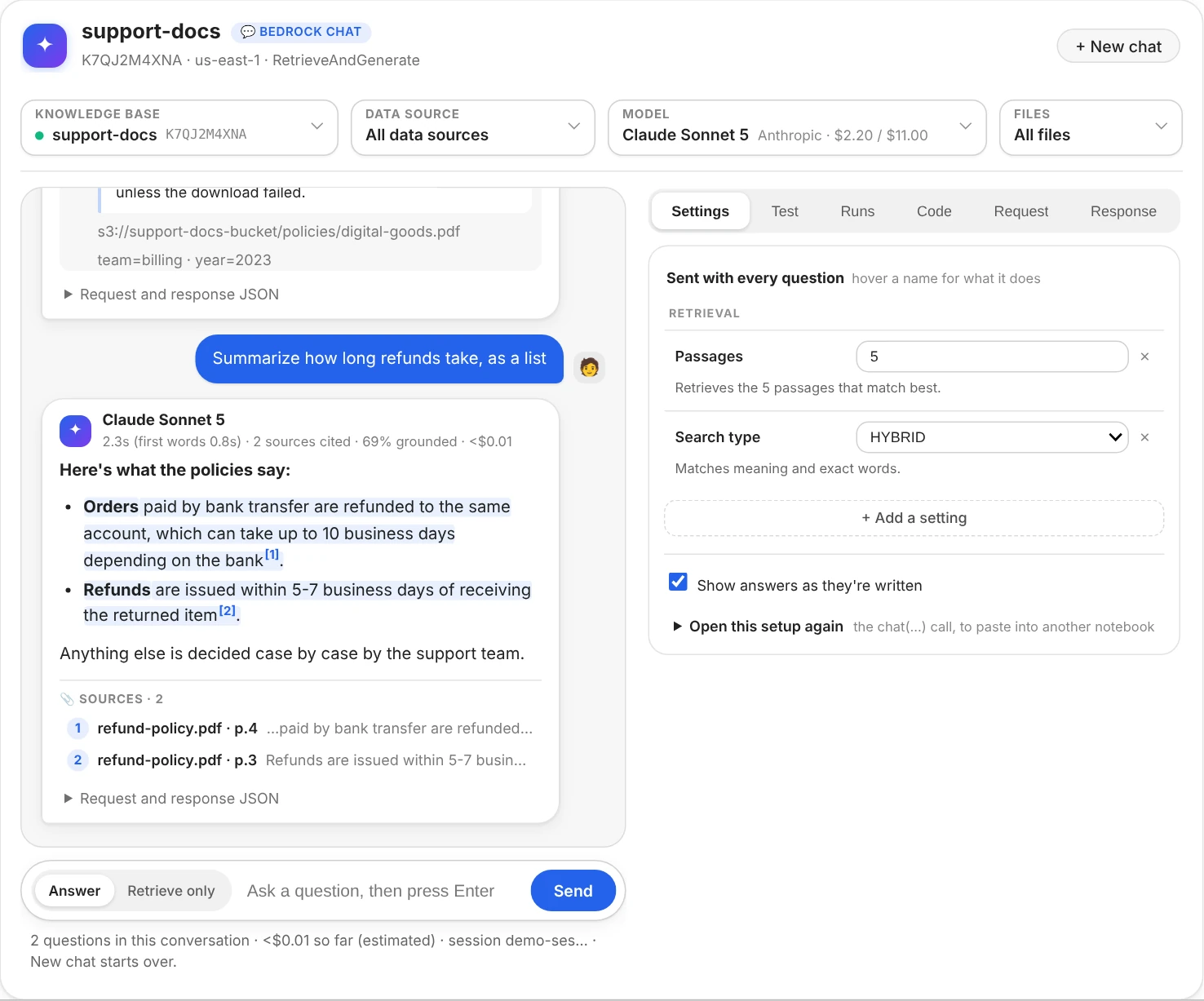
chat("support-docs", model="sonnet"): a question and a follow-up, each answer with its citations and sources, and the settings every question sends.
Quick start
from bedrock_chat import chat              # installed with pip: from aws_analyzer import chat

chat()                                     # pick the knowledge base and the model in the window
chat("support-docs", model="sonnet")       # or start on these: a name, ID or ARN; a model ID or short name
ui = chat("support-docs", n=8, temperature=0.2, search_type="hybrid", where={"team": "billing"})
The window needs ipywidgets, which SageMaker already has (elsewhere: %pip install ipywidgets, then reload the
browser tab). Without it, or outside Jupyter, every command below still works as a report.
- The conversation. Answers appear as they're written. Each one shades its cited spans and numbers them, lists
its sources (click one to read the passage, with its location and metadata), shows its time, grounded share and
estimated cost, and folds away the exact request and response. Findings under an answer say which setting to try
(Bedrock's "unable to assist" reply, no citations, a guardrail, cut off at
max_tokens). Follow-ups keep Bedrock's session; New chat starts over. - Settings. Everything sent with every question, each value explained in a sentence, with its path in the
request. Change it in place, remove it with ✕, add the common ones with one click, or add any field by its name
or path: the list comes from the installed boto3's description of the API, so nothing is missing. A value that
can't be sent turns red and says why, and warnings catch what Bedrock would refuse (
temperaturewithtop_pon a newer Claude model, a guardrail ID without its version, a prompt that drops the citation instructions). - Request JSON. The exact request the next question sends, as a folding tree with your settings highlighted, as plain JSON, or as the boto3 call to paste into your code. Edit JSON takes a hand-edited request back into the settings, after checking it the way boto3 does before sending. Last response shows what came back.
Commands (BedrockChatView)
chat() returns the view behind the window. Its commands share the window's settings and conversation, and an open
window follows them.
Chat
| Command | What it shows |
|---|---|
app() |
The chat window: knowledge base and model pickers, the conversation, and the Settings, Request JSON and Last response tabs |
ask(question) |
An answer as a report: [1][2] citations, cards (grounded share, sources cited, model, estimated tokens and cost, time), findings and the sources table. Each question follows up on the ones before it |
new_chat() |
Forgets the conversation: the next question starts a new Bedrock session. The settings stay |
transcript() |
The conversation so far, as a report that stays in the notebook when it's saved (the window doesn't) |
last() |
The last answer in full: every cited passage, the exact request and response as JSON, and the same call in Python |
Settings
| Command | What it shows |
|---|---|
settings() |
Every setting sent with every question, what its value means, where it goes in the request, warnings, and the chat(...) call that opens this setup again |
set(name=None, value=None, **values) |
Changes settings: set(temperature=0.2, n=8), or set("generationConfiguration.performanceConfig.latency", "optimized") for any field. None removes one |
unset(*names) |
Stops sending settings: unset("temperature", "top_p") |
fields(match=None) |
Every field RetrieveAndGenerate takes in this boto3: the name set() takes, its type and range, what it does and its path. fields("rerank") keeps those that mention it |
request(question=None) |
The exact JSON the next question sends, highlighted, with what Bedrock would refuse in it, and the same call in Python. Nothing is sent |
Knowledge base and model
| Command | What it shows |
|---|---|
use(kb=None, model=None) |
Switches the knowledge base (a new conversation) or the model (the same one) |
kbs() |
The knowledge bases in the region: name, ID, status, description and when each changed |
models(match=None) |
The models you can chat with: the ID to pass as model=, on demand or through an inference profile, and $ per 1M tokens |
Settings with short names
chat() and set() take these as keywords. The API's own names (maxTokens, overrideSearchType) and paths work
too, and values are forgiving ("0.2", "hybrid", JSON text or a Python dict).
| Name | What it does |
|---|---|
n |
Passages to retrieve, 1 to 100 (Bedrock's default is 5) |
search_type |
"HYBRID" (meaning and exact words) or "SEMANTIC" |
filter (or where) |
Only documents whose metadata matches: {"team": "billing"}, {"year": (">=", 2024)} (in JSON, [">=", 2024]), or a Bedrock RetrievalFilter. The same vocabulary as bedrock_kb.py's where= |
reranker, rerank_n |
Re-order the passages with "cohere" (Cohere Rerank 3.5) or "amazon" (Amazon Rerank 1.0), or a model ID, and keep the best rerank_n |
temperature, top_p |
Randomness, 0 to 1. Newer Claude models take one of the two |
max_tokens, stop |
The longest answer in tokens; up to 4 stop sequences |
prompt |
Your own prompt template. It needs $search_results$; keep $output_format_instructions$ or answers lose their citations. Adding it in the window starts from bedrock_chat.DEFAULT_PROMPT |
model_fields |
The model's own settings, passed as they are: {"top_k": 50} for Claude |
guardrail_id, guardrail_version |
A Bedrock guardrail that screens the question and the answer |
latency |
"optimized" for latency-optimized inference, where the model offers it |
query_decomposition |
True: Bedrock splits a complicated question into simpler searches |
orchestration_prompt |
The prompt of the step that rewrites the question before searching |
kms_key |
A KMS key that encrypts the conversation Bedrock keeps |
Every other field goes by its path from knowledgeBaseConfiguration, e.g.
set("orchestrationConfiguration.inferenceConfig.textInferenceConfig.temperature", 0).
Reference
Getting the data (BedrockChatAnalyzer): requests and answers as Python objects
a = ui.answers[-1]                    # Answer: the conversation's answers, oldest first
a.text, a.citations, a.sources, a.grounded_share
a.request, a.response                 # exactly what was sent and what came back
a.to_df()                             # one row per cited source
ui.values                             # the settings: {'n': 8, 'temperature': 0.2, ...}

core = ui.core                        # or BedrockChatAnalyzer(region="us-west-2", profile="dev")
params = core.request("support-docs", "refund window?", {"n": 8})        # the request, without sending it
a = core.ask("support-docs", "refund window?", {"n": 8, "temperature": 0.2}, model="sonnet")
a = core.ask("support-docs", "and for EU orders?", session_id=a.session_id)  # a follow-up
core.ask("support-docs", "refund window?", stream=True, on_text=show)    # show(text) gets the answer so far
core.schema().fields["temperature"]   # Field: path, type, range, what it does
The analysis functions don't call AWS: request_schema, normalize_settings, coerce_setting, build_request,
settings_from_request, validate_request, python_call, parse_rag, collect_stream, as_filter,
describe_filter, describe_setting, answer_cost, and the findings: settings_findings and answer_findings.
Cost and limits: how answers are priced
- RetrieveAndGenerate doesn't report tokens, so they're estimated from characters (the question, the prompt and the passages retrieved; only the cited ones come back, so their average size stands in for the rest) and labelled as estimates. The estimate adds the question's embedding and, with a reranker, the reranking.
- Prices are the same us-east-1 list prices as
bedrock_kb.py(MODEL_PRICES,GLOBAL_MODEL_PRICES,BEDROCK_PRICES); pass your own withBedrockChatAnalyzer(model_prices={...}, prices={...}). A model that isn't in the table shows its cost as unknown. - Bedrock takes questions of up to 1,000 characters; the chat says so before sending a longer one.
IAM permissions: read-only, and what needs which
| Permission | Used by |
|---|---|
bedrock:ListKnowledgeBases |
The knowledge base picker, kbs, and finding a knowledge base by name |
bedrock:RetrieveAndGenerate and bedrock:Retrieve on the knowledge base, bedrock:InvokeModel on the model or inference profile |
Asking, in the window or with ask. Streamed answers (RetrieveAndGenerateStream) use the same permission; where streaming is refused anyway, answers arrive all at once and the window says why |
bedrock:ListFoundationModels, bedrock:ListInferenceProfiles |
The model picker, models, and turning model="sonnet" into an ID |
A model also has to be enabled under Model access in the Bedrock console. A list the role can't read becomes a box to type into instead of a picker, with a note naming the missing permission. The chat guide has a ready-made IAM policy.
Amazon SageMaker
The notebook you're running in, and everything else SageMaker bills you for. What this notebook is and what it costs, whether it stops when idle, how busy its CPU, memory, disk and GPU are, what fills its disk, and which notebooks, apps and endpoints in the region look forgotten.
📄 analyzers/sagemaker_env.py · 📖 SageMaker guide
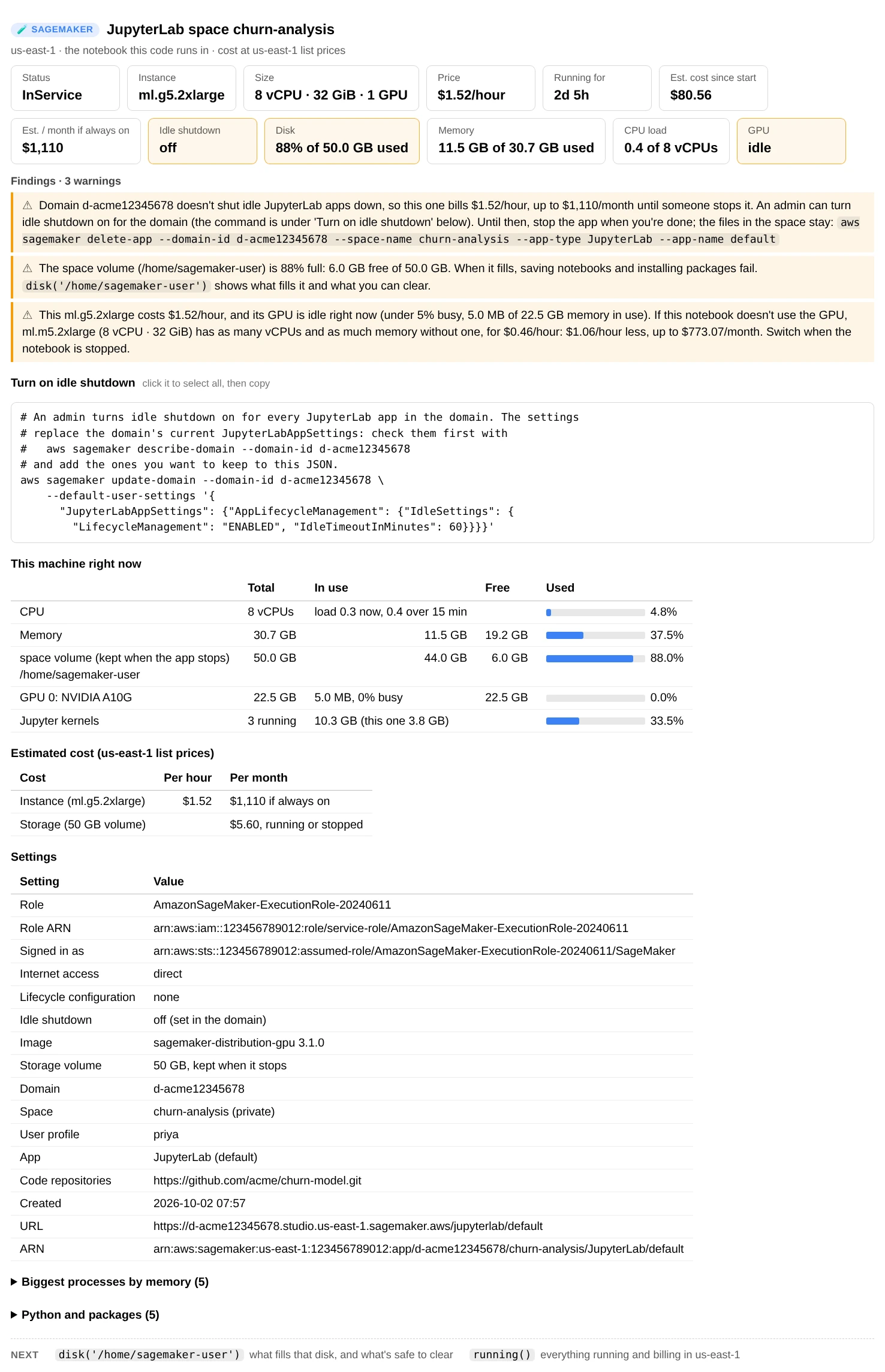
ui.instance() in a Studio JupyterLab space: about $80 spent so far on a GPU that has sat idle, and nothing will stop the app tonight.
The file isn't called sagemaker.py, so it doesn't hide the SageMaker Python SDK, which is also imported as
sagemaker.
Quick start
Every command works with boto3 alone, so on SageMaker there's nothing to install.
from sagemaker_env import SageMakerView

ui = SageMakerView()             # uses the notebook's execution role and region
ui.help()                        # every command, grouped by task

ui.instance()                    # this notebook: type, cost so far, idle shutdown, CPU / memory / disk / GPU now
ui.disk()                        # what fills the disk, and the caches and trash that are safe to clear
ui.running()                     # everything billing by the hour in the region, and what looks forgotten
ui.instance("old-experiment")    # another notebook instance, or a Studio space by name
NOTE:
instance()anddisk()read the machine they run on, so run them in the notebook you want to know about: a notebook instance, or a Studio JupyterLab, Code Editor or Studio Classic app. Anywhere else,instance("name")andrunning()still work. Nothing in the file stops, deletes or changes anything; where that would help, the report shows the command.
Commands (SageMakerView)
Grouped the way ui.help() lists them.
This notebook
| Command | Shows |
|---|---|
instance(name=None) |
The notebook you're in: instance type with its vCPUs, memory and GPUs, price per hour, how long it has run and what that cost, what a month of it costs if it's never stopped, and whether anything stops it when idle (a notebook instance's auto-stop lifecycle configuration, or the Studio domain's idle shutdown), with the commands that turn it on. Then the machine right now: CPU load, memory, each disk and whether it survives a stop, GPU memory and use, the Jupyter kernels and the memory they hold, the biggest processes, and the Python and package versions. Settings: role, network, lifecycle configuration, image or platform, storage volume, space and domain. Findings: no idle shutdown, a disk or memory nearly full (and the other kernels holding memory), an idle GPU (and the CPU type with the same vCPUs and memory, with the saving), an instance far bigger than what's in use, Amazon Linux 1. name= shows another notebook instance or Studio space ("d-abc123/analysis" when two domains have one), without its machine |
disk(path=None, top=20, limit="200k") |
How full the disk is and what fills it: the biggest folders as a tree three levels deep, the biggest files and when they last changed, and the caches and trash that are safe to clear (Jupyter's trash, pip and conda caches, Hugging Face and PyTorch downloads, notebook checkpoints), each with the command that empties it. Findings: a nearly full disk (with the command that makes the volume bigger and what that costs a month), what can be cleared, big files untouched for 90 days (and what they'd cost in S3). The default folder is where your notebooks live: ~/SageMaker on a notebook instance, /home/sagemaker-user in Studio |
Your account
| Command | Shows |
|---|---|
running(metrics=True, days=7) |
Everything SageMaker bills by the hour in the region: notebook instances, Studio apps (JupyterLab, Code Editor, Studio Classic), endpoints, and training and processing jobs, with the instance, price per hour, how long each has run and whether it stops when idle, and each endpoint's requests over the last days days from CloudWatch. Stopped notebook instances are listed too, because their volumes are still billed. Findings, each with the command that stops it: notebooks and apps running for over 12 hours with nothing to stop them, endpoints with no requests, and the storage that stopped notebook instances keep |
Reference
Getting the data (SageMakerAnalyzer): the notebook, the machine and what's running, as Python objects
ui.core is the SageMakerAnalyzer. Every UI command has a data method on it:
sm = ui.core                                          # or SageMakerAnalyzer(region="eu-west-1", profile="dev")

report = sm.instance()                                # InstanceReport: .env, .notebook, .machine, .identity
report.notebook.instance_type, report.notebook.idle   # 'ml.g5.2xlarge', 'off'
report.machine.memory_share, report.machine.gpus      # 0.37, [GPUInfo(name='NVIDIA A10G', busy=0.0, ...)]
sm.notebook("old-experiment")                         # NotebookInfo for any notebook instance or Studio space
sm.environment()                                      # Environment: where this code runs, from SageMaker's metadata
sm.machine()                                          # Machine: this machine right now (local reads only)

d = sm.disk("~/SageMaker", limit=None)                # DiskReport: folders, largest files, caches you can clear
d.to_df()                                             # one row per folder

r = sm.running(days=30)                               # RunningReport: .resources, .stopped, .errors
r.to_df()                                             # one row per notebook, app, endpoint and job
The analysis functions are pure (no AWS calls), so they also work on responses you already have:
parse_metadata, parse_notebook_instance, parse_app, apply_studio_settings, studio_idle, lifecycle_idle,
parse_endpoint, parse_training_job, parse_processing_job, parse_meminfo, parse_loadavg, parse_gpus,
parse_process, hourly_price, describe_instance, notebook_costs, smaller_type, folder_tree,
idle_shutdown_commands, stop_command, and the findings: instance_findings, disk_findings, running_findings.
Cost and limits: the prices used, and what's measured and what's estimated
- Costs are estimates at us-east-1 on-demand list prices, read from the AWS Price List API on 2026-09-27.
INSTANCE_TYPESholds the price per hour of 134 instance types, with their vCPUs, memory and GPUs; a type costs the same per hour as a notebook instance, a Studio app, an endpoint or a job.SAGEMAKER_PRICESadds storage per GB-month: $0.14 for a notebook instance's volume, $0.112 for a Studio space's, and S3 Standard's $0.023 to compare with. For another region or a discount, pass your own:SageMakerAnalyzer(prices={"ml.g5.xlarge": 1.21, "notebook_storage": 0.15}). A type that isn't in the table shows its cost as unknown, and every report says whether it used list prices or yours. - "Cost since start" is the price per hour times how long it has run: since boot for the notebook instance you're in, since the app started for a Studio app, and since its last change (about when it last started) for any other notebook instance. Spot training jobs cost less than the on-demand price shown.
instance()reads CPU load (the 15-minute average) and memory as they are now, so the suggestion of a smaller instance says "if that's typical". Whether a notebook instance stops when idle is read from its lifecycle configuration script: AWS's auto-stop-idle sample and scripts like it.disk()stops after 200,000 files by default and says so (limit=Nonemeasures everything). It stays on one disk and doesn't follow links.
IAM permissions: read-only, and which command needs which
Read-only, per command:
| Permission | Used by |
|---|---|
sagemaker:DescribeNotebookInstance, sagemaker:DescribeNotebookInstanceLifecycleConfig |
instance on a notebook instance, running |
sagemaker:DescribeApp, sagemaker:DescribeSpace, sagemaker:DescribeDomain, sagemaker:DescribeUserProfile |
instance in Studio; running reads the domains |
sagemaker:ListDomains, sagemaker:ListSpaces, sagemaker:ListApps |
instance("space name") |
sagemaker:ListNotebookInstances, sagemaker:ListApps, sagemaker:ListEndpoints, sagemaker:DescribeEndpoint, sagemaker:DescribeEndpointConfig, sagemaker:ListTrainingJobs, sagemaker:DescribeTrainingJob, sagemaker:ListProcessingJobs, sagemaker:DescribeProcessingJob |
running |
cloudwatch:GetMetricData |
running: endpoint requests |
sts:GetCallerIdentity (who you're signed in as) needs no permission, and disk() only reads local files. Anything
you can't read shows up as a note instead of an error. The AmazonSageMakerFullAccess managed policy, which many
execution roles have, includes the sagemaker: permissions. The
SageMaker guide has a ready-made IAM
policy that covers every command.
Development
pip install -r requirements-dev.txt    # pinned versions
python -m pytest                       # every test, no AWS account needed
ruff check .                           # lint
python -m build                        # the PyPI package, in dist/

pip install -r requirements-docs.txt   # the guide site
mkdocs serve                           # preview it at http://127.0.0.1:8000
- Tests run against moto, so no AWS account is needed. moto covers little of
Bedrock and none of SageMaker Studio, so the Bedrock Knowledge Bases tests and the SageMaker Studio and
running()tests use botocore'sStubberon real clients instead, which also checks every request against the service model. The SageMaker tests read a fake machine (metadata file,/proc, a home folder) from a temporary folder. The chat window's tests click its ipywidgets in Python, against fake Bedrock clients that check every request, response and stream event against the service model. - Guides in
docs/are Markdown, built with MkDocs and the Material theme (mkdocs.yml) and published to GitHub Pages by the Docs workflow whenever they change onmain; pull requests build them with--strict, so a broken link fails there.docs/index.mdis the home page with a card per service, and each service has its own guide (docs/s3.md,docs/dynamodb.md,docs/bedrock_kb.md,docs/bedrock_chat.md,docs/sagemaker_env.md); a new analyzer gets a new guide, a card on the home page and an entry inmkdocs.yml'snav. - Screenshots are the tool's own output from demo buckets, tables and knowledge bases with synthetic data;
.claude/skills/demo/shots.pyremakes them (it needs Pillow and a headless Chrome), and.claude/skills/demo/demo.pyruns any command against the same kind of data. Bedrock's are served by a simulated Bedrock, since moto has none. The chat window's are taken in a real JupyterLab by.claude/skills/demo/chat_shots.py(it needs jupyterlab and playwright too). - The PyPI package (
pyproject.toml) shipsanalyzers/*.pyunchanged as the modules of theaws_analyzerpackage;src/aws_analyzer/__init__.pyonly re-exports the classes and holds__version__. Optional packages are extras:data(pandas, pyarrow),files(Excel, PDF, .zst, snappy),notebook(IPython, ipywidgets, tqdm) andall. To release, bump__version__and publish a GitHub release taggedv<version>: the Release workflow builds it, checks it and uploads it to PyPI with trusted publishing (its comments have the one-time setup). - CI runs the same checks on Python 3.10 to 3.14 for every pull request and push to
main, and also imports each analyzer on its own with only boto3 installed, and builds the package and imports it the same way. The versions inrequirements-dev.txtandrequirements-docs.txtare pinned; Dependabot opens weekly pull requests to update them and the GitHub Actions the workflows use.
License
1 maintainer

Metadata
1 maintainer
Release files for aws-analyzer 0.1.0
For a detailed explanation of source distributions (sdists) and built distributions (wheels), please see the package formats documentation.
Source distribution (sdist)
| File | Size | Uploaded | |
|---|---|---|---|
| aws_analyzer-0.1.0.tar.gz | 523.2 kB | Details |
Built distribution (wheel)
| File | Interpreter | ABI | Platform | Reset |
|---|---|---|---|---|
| aws_analyzer-0.1.0-py3-none-any.whl | Python 3 | none | any | Details |
Total release size: 914.6 kB
Release files / aws_analyzer-0.1.0.tar.gz
| Download URL | aws_analyzer-0.1.0.tar.gz |
|---|---|
| Size | 523.2 kB |
| Tags | Source |
|
SHA-256 checksum How to use checksums |
c42265a55dc2d49df7e19ff69a1b8c24689bfae215198d22b77d42e2518df429
|
|
BLAKE2b-256 checksum How to use checksums |
5eb1250c1b71883dfce736762720a76b4b48d886b575ec7d25e1cc6963192812
|
| Upload date | |
|
Uploaded using Trusted Publishing? What is trusted publishing? |
Yes |
| Uploaded via |
twine/7.0.0 CPython/3.13.14
|
Provenance
Provenance describes where a file came from. On PyPI, provenance is shared via attestations, which provide a verifiable record of the build or publishing details. View details, limitations and caveats.


PyPI Publish Attestation
PyPI verified that this artifact, at this checksum, originated from the publisher listed below.
Signed by GitHub Actions, verified by PyPI on Oct 4, 2026.
Transparency logRelease files / aws_analyzer-0.1.0-py3-none-any.whl
| Download URL | aws_analyzer-0.1.0-py3-none-any.whl |
|---|---|
| Size | 391.4 kB |
| Tags | Python 3 |
|
SHA-256 checksum How to use checksums |
6eabff7fdb5bc4a14afac8b1a3345587d93be4a131777384187de2e6b341f88b
|
|
BLAKE2b-256 checksum How to use checksums |
c4394d454cdaf42de488f37a0f578485e788682d9a735e2835688f8cc6b13a3f
|
| Upload date | |
|
Uploaded using Trusted Publishing? What is trusted publishing? |
Yes |
| Uploaded via |
twine/7.0.0 CPython/3.13.14
|
Provenance
Provenance describes where a file came from. On PyPI, provenance is shared via attestations, which provide a verifiable record of the build or publishing details. View details, limitations and caveats.
PyPI Publish Attestation
PyPI verified that this artifact, at this checksum, originated from the publisher listed below.
Signed by GitHub Actions, verified by PyPI on Oct 4, 2026.
Transparency log













