Parametric modeling, analysis, and multidisciplinary design optimization of axial-flux permanent-magnet motors
Verified details
These details have been verified by PyPIProject links
GitHub Statistics
Maintainers

Project description
axfluxmdo
Open-source Python toolkit for parametric modeling, simulation, visualization, and multidisciplinary design optimization of axial-flux permanent-magnet motors.


axfluxmdo is a reusable science layer that sits above expert motor designers and
high-fidelity FEA — not a replacement for either. It provides parametric axial-flux
geometry, fast analytical physics models, constraint visualization, and (in later phases)
solver automation and Pareto-front optimization, so that design tradeoffs can be explored
systematically instead of by intuition-only iteration.
Phases 1–4 (current): the analytical workbench (parametric motor object, energy-consistent torque/back-EMF/loss/thermal model, constraints, sweeps, geometry visualization), the 2.5D annular slice model (radius-resolved fields and losses, manufacturing imperfections, torque-ripple and axial-force metrics, efficiency maps), the MDO layer (pymoo Pareto optimization over mixed continuous/discrete variables, OpenMDAO integration, sensitivity tornado charts), and external solver hooks (Gmsh mesh export, a GetDP magnetostatics pipeline, and sim-to-analytical residual analysis). Evaluating a design takes microseconds, so a full Pareto study runs in seconds — and the analytical layer's error budget is quantified against open-source FEA.
Install
pip install axfluxmdo                  # core (analytical + annular models, 2D viz)
pip install "axfluxmdo[opt]"           # + pymoo / OpenMDAO / scikit-learn optimization
pip install "axfluxmdo[fea]"           # + gmsh mesh export (GetDP is a separate binary)
pip install "axfluxmdo[viz3d]"         # + PyVista 3D rendering/animations
For development:
git clone https://github.com/jman4162/axfluxmdo.git
cd axfluxmdo
pip install -e ".[dev,opt,fea,viz3d]"
Quickstart
from axfluxmdo import AxialFluxMotor, OperatingPoint
from axfluxmdo.models import AnalyticalModel
from axfluxmdo.viz import plot_geometry

motor = AxialFluxMotor(
    outer_radius=0.08,      # m
    inner_radius=0.025,     # m
    air_gap=0.0008,         # m
    pole_pairs=14,
    phases=3,
    turns_per_phase=24,
    fill_factor=0.45,
    magnet_thickness=0.004,        # m
    back_iron_thickness=0.006,     # m
)

op = OperatingPoint(speed_rpm=500, current_rms=25, dc_bus_voltage=48)

result = AnalyticalModel().evaluate(motor, op)
print(result)
plot_geometry(motor, show=True)
AnalyticalResult
  torque:            8.629 N·m
  torque density:    2.364 N·m/kg
  back-EMF (rms):    6.02 V/phase
  elec frequency:    116.7 Hz
  air-gap B:         1.016 T
  current density:   4.04 A/mm²
  copper loss:       20.0 W
  core loss:         0.91 W
  efficiency:        0.9557
  winding temp:      49.6 °C
  mass:              3.651 kg
  constraints:
    winding_temp_c: 49.57 <= 140 [OK, margin +64.6%]
    electrical_frequency_hz: 116.7 <= 1000 [OK, margin +88.3%]
    current_density_a_mm2: 4.042 <= 10 [OK, margin +59.6%]
    line_voltage_v: 10.9 <= 33.94 [OK, margin +67.9%]
    core_flux_density_t: 0.6696 <= 1.6 [OK, margin +58.2%]
    magnet_temp_c: 65 <= 80 [OK, margin +18.8%]
Pole-pair tradeoff in four lines
from axfluxmdo.sweeps import sweep_pole_pairs

sweep = sweep_pole_pairs(motor, op, pole_pairs=range(4, 21, 2))
sweep.plot(show=True)
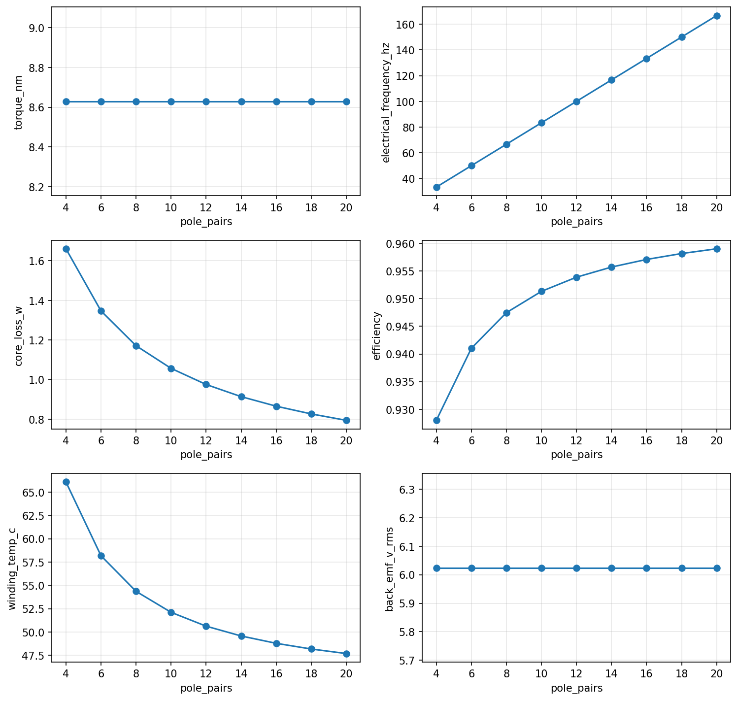
At fixed air-gap field and electrical loading, torque is independent of pole count — the
real tradeoff is yoke saturation at low p (p = 4 is infeasible here: the fixed stator
core would need to carry 2.3 T) versus electrical frequency, switching burden, and ripple
at high p. See examples/ for executed notebooks.
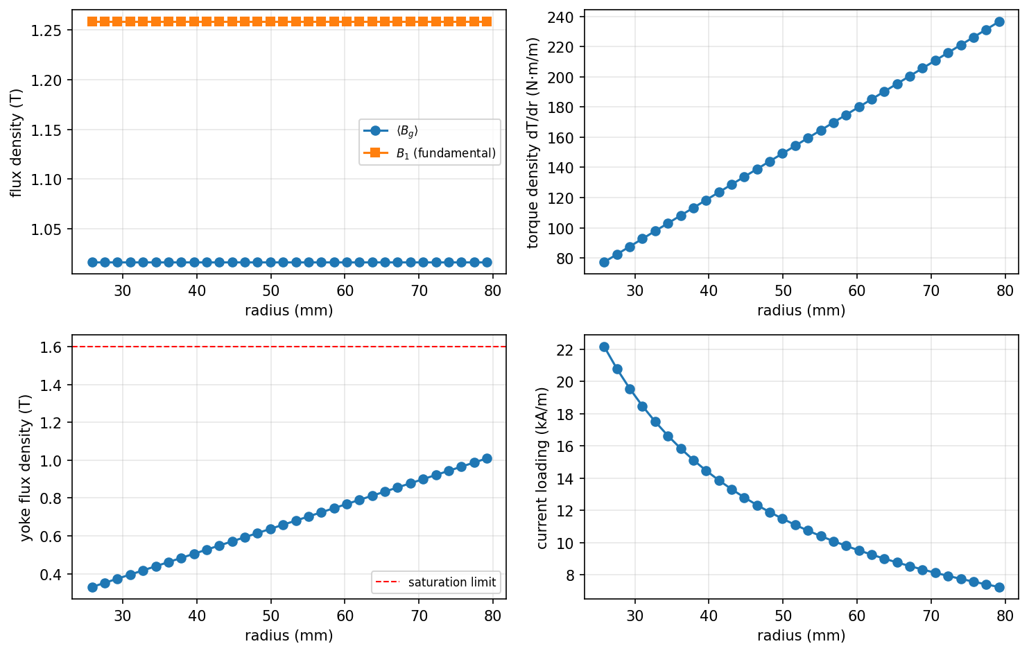
The 2.5D annular model (Phase 2)
import dataclasses
from axfluxmdo import GapImperfections
from axfluxmdo.models import AnnularModel, compute_efficiency_map
imperfect = dataclasses.replace(
motor,
tolerances=GapImperfections(gap_offset_m=1e-4, coning_m=2e-4, runout_m=3e-4),
magnet_shape="rectangular",
)
result = AnnularModel(n_slices=32).evaluate(imperfect, op)
print(result.torque_ripple_proxy, result.axial_force_n)
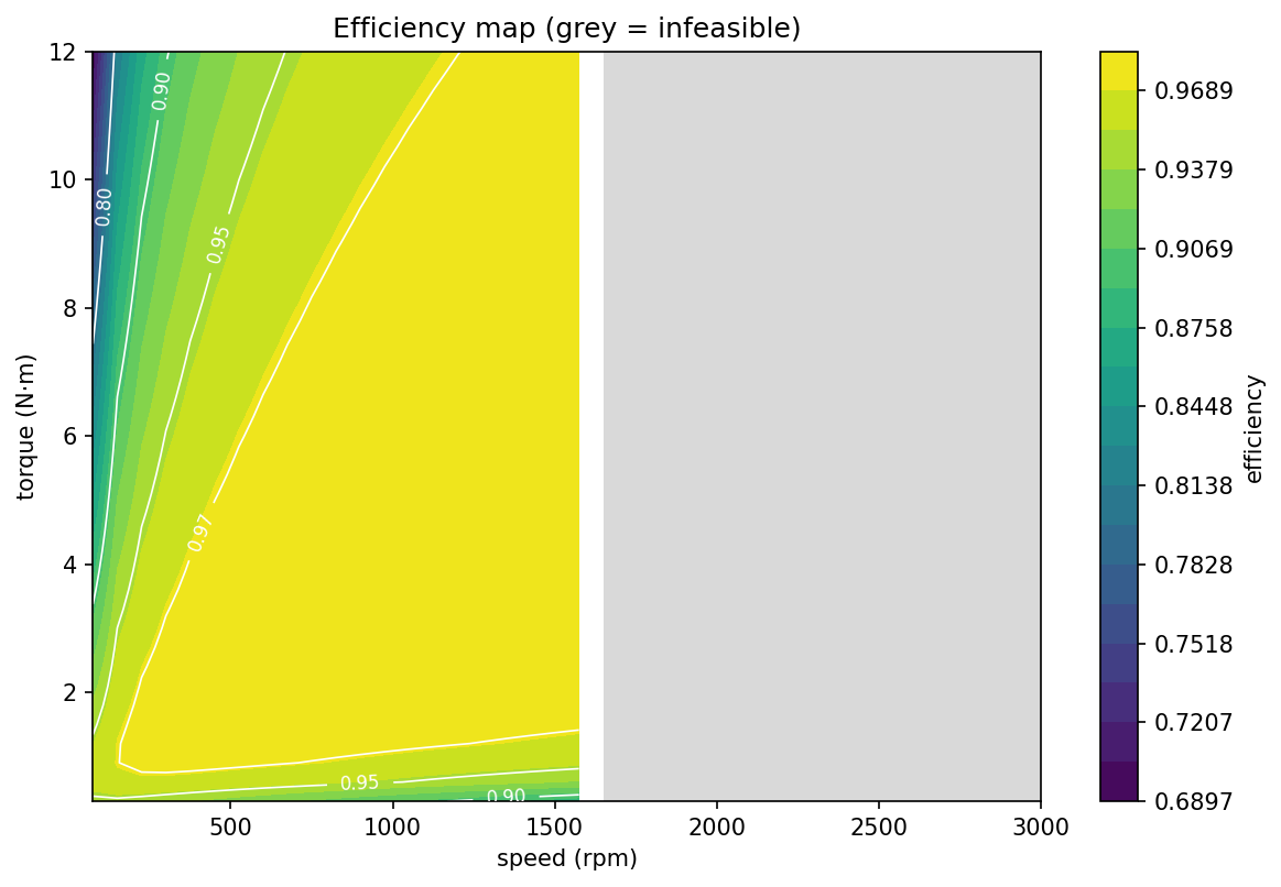
emap = compute_efficiency_map(motor, op, max_speed_rpm=3000, max_torque_nm=12)
emap.plot(show=True)
The disk machine is split into radial annuli; torque and back-EMF derive from the same summed flux linkage, so for a perfect machine the annular model agrees with the analytical layer to machine precision (pinned by tests) — added fidelity appears only where physics is genuinely radius-dependent:
- Yoke saturation binds at the outer radius (pole pitch widens with r); the mean-radius proxy of Layer 1 underestimates it.
- Manufacturing imperfections: uniform gap error, rotor coning (gap varying with radius), and runout (1/rev gap oscillation, averaged analytically — the load line is convex in the gap, so mean torque rises slightly with runout; the real penalties are the 1/rev ripple proxy and the multi-kN axial-force modulation).
- Constraint-aware efficiency maps over the speed–torque plane, with the binding constraint recorded for every infeasible cell.
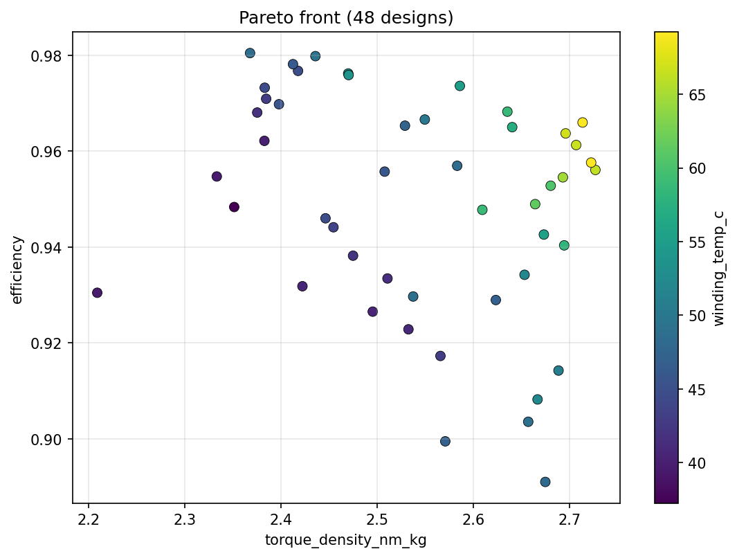
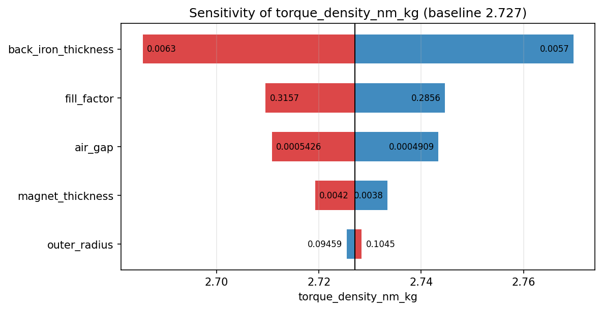
Pareto optimization (Phase 3)
Requires the optimization extra: pip install -e ".[dev,opt]" (pymoo + OpenMDAO).
from axfluxmdo.optimize import optimize_pareto
from axfluxmdo.viz import plot_pareto

study = optimize_pareto(
    motor,
    op,
    variables={
        "outer_radius": (0.05, 0.12),
        "pole_pairs": [8, 10, 12, 14, 16, 18, 20],
        "air_gap": (0.0005, 0.0015),
        "fill_factor": (0.30, 0.60),
    },
    objectives=["maximize_torque_density", "maximize_efficiency", "minimize_mass"],
    constraints=["winding_temp_c < 140", "electrical_frequency_hz < 1000"],
)

plot_pareto(study, x="torque_density", y="efficiency", color="winding_temp_c", show=True)
Mixed continuous/discrete variables run through pymoo's MixedVariableGA; the model's
built-in limits (thermal, voltage, current density, saturation, magnet temperature) are
enforced in addition to the user constraint strings, so every returned design is
feasible. One-at-a-time sensitivities (compute_sensitivities + plot_tornado) show
which variables actually move a chosen design, and an OpenMDAO ExplicitComponent
wrapper supports gradient-based refinement and larger coupled MDO groups.
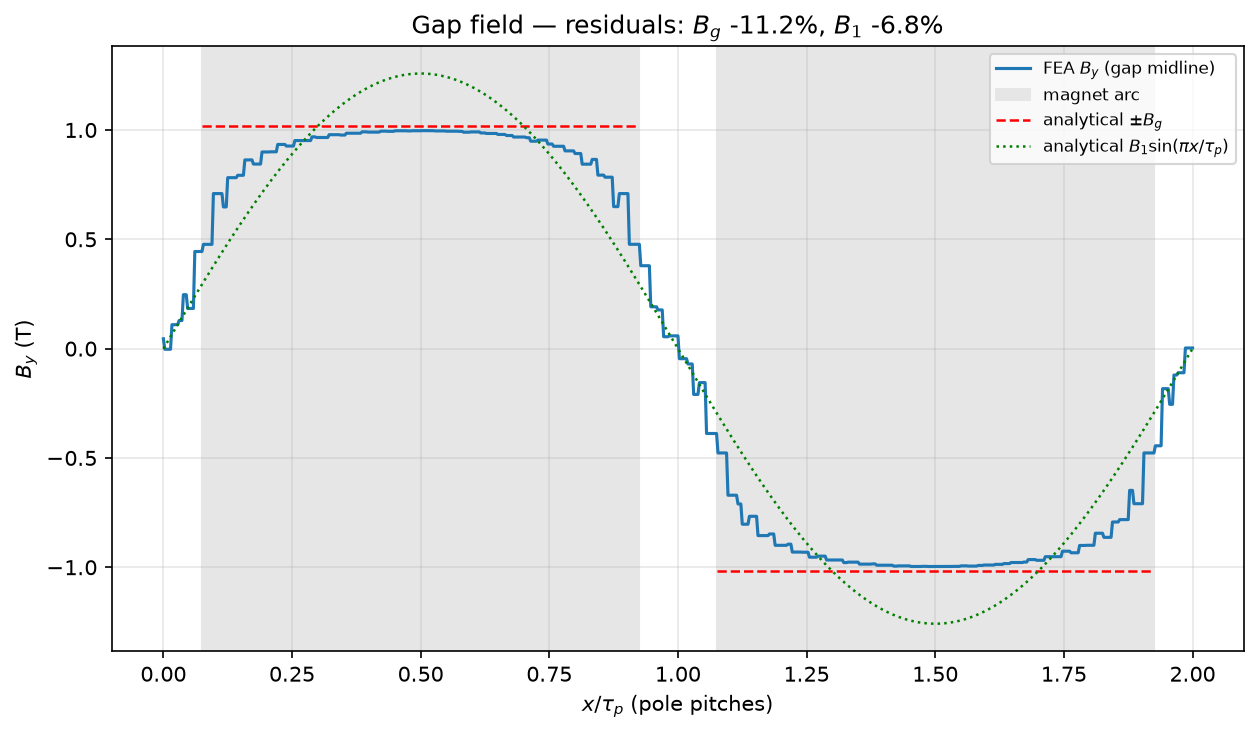
FEA validates the analytical layer (Phase 4)
from axfluxmdo.solvers import solve_open_circuit          # needs getdp on PATH
from axfluxmdo.validation import compare_open_circuit, measured_carter_factor

slotless = solve_open_circuit(motor, magnet_temp_c=65.0)  # gmsh -> GetDP -> parsed field
slotted = solve_open_circuit(motor, slotted=True, magnet_temp_c=65.0)
print(compare_open_circuit(motor, slotless, magnet_temp_c=65.0))
print(measured_carter_factor(slotless, slotted, motor))
The annulus is unrolled at the mean radius into a 2D planar magnetostatics problem
(one pole pair, periodic), meshed by Gmsh (pip install "axfluxmdo[fea]") and
solved open-circuit by GetDP (external binary; tests and examples degrade
gracefully without it — committed golden results keep the figures reproducible).
The FEA shares the load line's exact recoil-line magnet model, so residuals isolate
geometry that the 1D circuit cannot see. Measured on the reference motor
(GetDP 3.5.0):
- the load line overestimates: FEA's under-magnet mean is −11.2% vs B_g and the fundamental is −6.8% vs B₁ — inter-magnet leakage and gap fringing;
- slotting knocks the field down a further 7.6%, giving a measured Carter factor
k_C = 1.44; feeding it back into
airgap_flux_density(..., carter_factor=k_C)reproduces the FEA slotless/slotted ratio to 4 decimals.
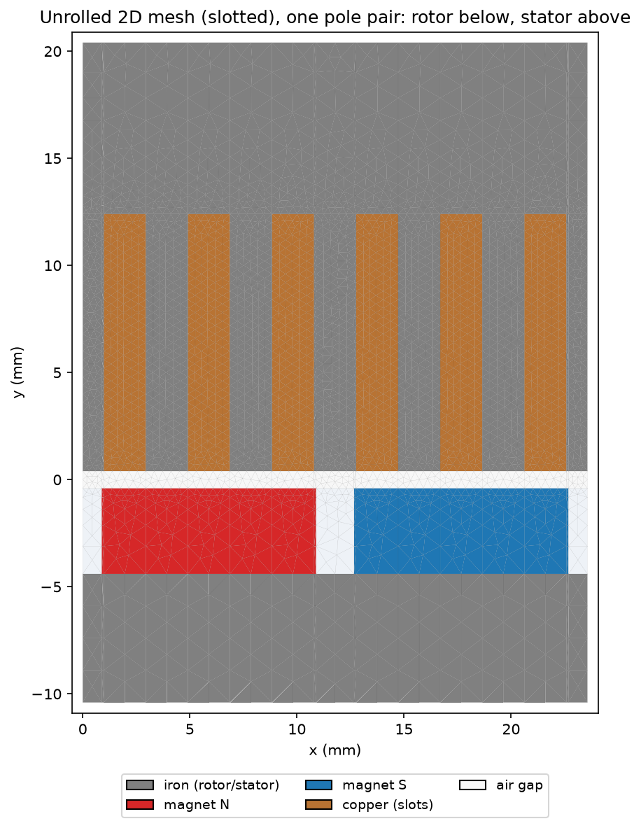
A 3D annular-sector mesh export (export_3d_sector) is included for downstream
tooling; Elmer integration is deferred.
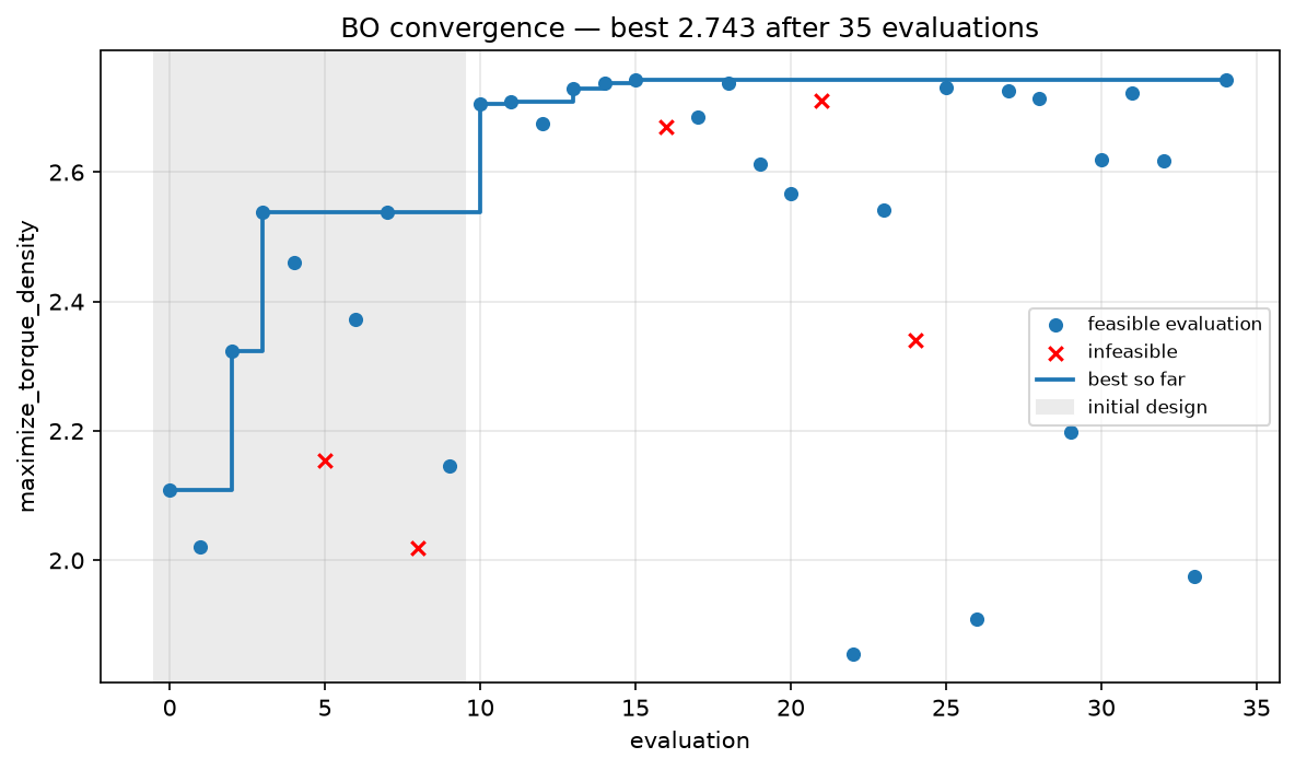
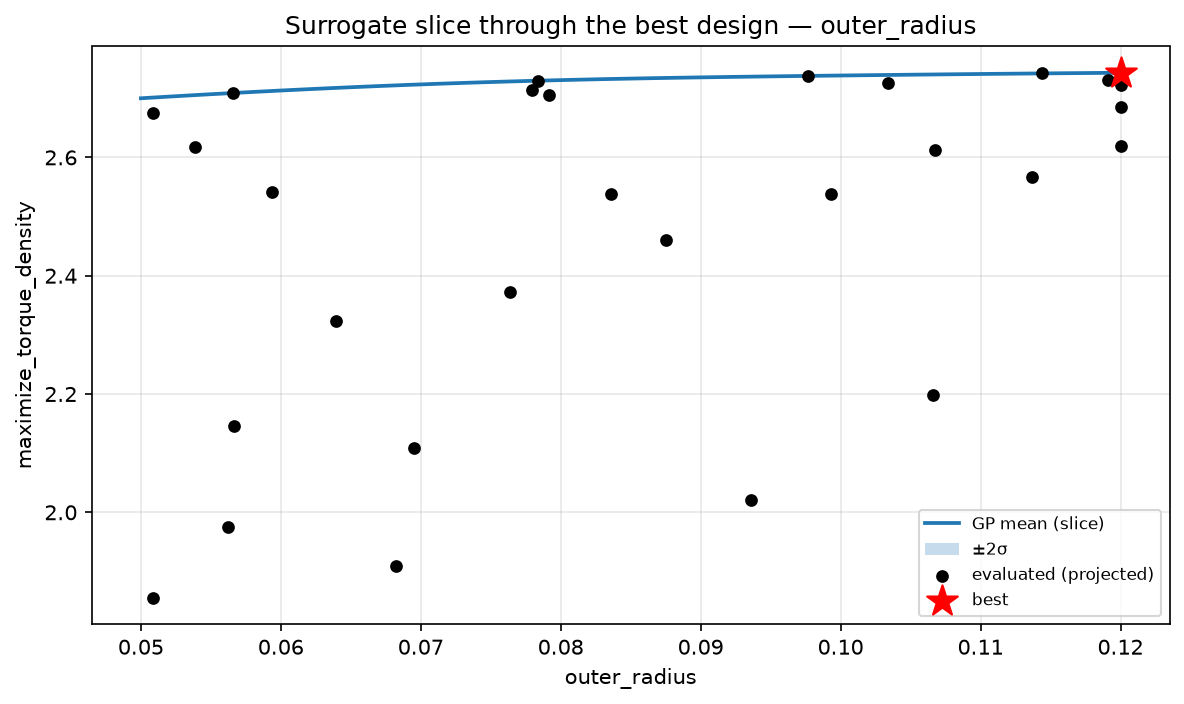
Bayesian optimization for expensive evaluations (Phase 5)
from axfluxmdo.optimize import bayesian_optimize

study = bayesian_optimize(
    motor,
    op,
    variables={
        "outer_radius": (0.05, 0.12),
        "air_gap": (0.0005, 0.0015),
        "fill_factor": (0.30, 0.60),
        "pole_pairs": [8, 10, 12, 14, 16, 18, 20],
    },
    objective="maximize_torque_density",
    constraints=["winding_temp_c < 140", "electrical_frequency_hz < 1000"],
    n_initial=10,
    n_iterations=25,
    seed=42,
)
print(study.summary())
print(study.recommend(k=3))   # uncertainty-aware: ranked by surrogate mean − σ
A Gaussian-process surrogate (ARD Matérn, scikit-learn) plus expected-improvement
acquisition finds the example-05 torque-density champion's neighborhood in 35
evaluations instead of the GA's ~1200 — the regime that matters when each evaluation
is a FEA solve or a dyno run. An expensive_fn hook plugs any costly objective into
the loop (e.g. a live GetDP solve from Phase 4); every evaluation lands in a
persistable DesignDataset (JSON Lines), and recommendations are ranked by the
surrogate's pessimistic estimate so unverified corners of the space don't win on
optimism.
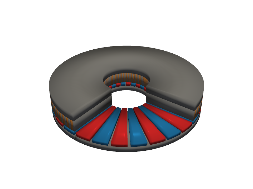
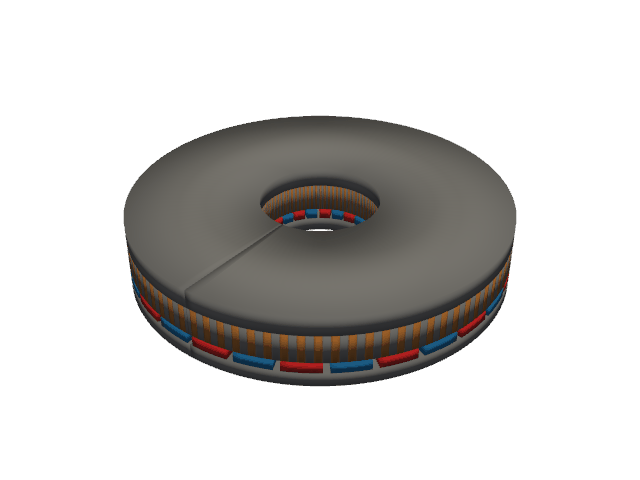
3D visualization
from axfluxmdo.viz import plot_motor_3d, animate_rotation, animate_exploded

plot_motor_3d(motor, show=True)                      # interactive cutaway view
animate_rotation(motor, "rotation.gif")              # rotor spinning over the stator
animate_exploded(motor, "exploded.gif")              # assembly exploding/reassembling
The parametric motor renders as a true 3D assembly via PyVista
(pip install "axfluxmdo[viz3d]"): rotor back iron, alternating N/S magnets, the
slotted stator with copper coils, and the yoke — every solid built from the same
AxialFluxMotor dimensions the physics models use (mesh volumes match the analytic
volume properties to <0.1%, tested).

What's in the model (Phase 1)
- Magnetics: magnet load-line air-gap flux density with temperature-derated
remanence, fundamental-harmonic flux linkage; torque and back-EMF derived from the same
flux linkage so the power balance
m·E·I = T·ωholds to machine precision (enforced by tests). - Losses: copper loss with resistance–temperature coupling, two-term Steinmetz core loss (M-19 coefficients pinned to datasheet values), mechanical-loss placeholder.
- Thermal: closed-form steady-state lumped RC winding temperature including the copper-loss/temperature fixed point, with thermal-runaway detection.
- Constraints: winding temperature, electrical frequency, current density, inverter voltage, yoke saturation, magnet temperature — each reported with normalized margin.
- Materials: NdFeB grades (N35/N42/N48/N42SH), M-19 29ga steel, copper.
- Sweeps & viz: one-line parameter sweeps over any design field, front-view and cross-section geometry plots.
Development
pip install -e ".[dev]"
pytest                       # full suite
ruff check . && ruff format --check .
Roadmap
All five SPEC phases are shipped.
| Phase | Scope | Status |
|---|---|---|
| 1 | Analytical workbench: parametric motor, torque/EMF/losses/thermal RC, constraints, pole-pair sweep, geometry viz | ✅ |
| 2 | 2.5D annular slice model: radius-dependent flux/loading/losses, air-gap & runout sensitivity, efficiency maps | ✅ |
| 3 | MDO: OpenMDAO components, pymoo Pareto optimization, sensitivity analysis | ✅ |
| 4 | External solver integration: Gmsh export, GetDP pipeline, sim-to-analytical residuals (Elmer deferred) | ✅ |
| 5 | Surrogates & Bayesian optimization for expensive design loops | ✅ |
Model fidelity & known limitations
The fast layers are deliberately simple; know what they leave out before trusting absolute numbers (all of these are also documented at the relevant docstrings):
- Single-gap topology (one rotor, one stator). Real axial-flux machines are often
double-gap (TORUS/YASA/AFIR); the single-sided rotor carries a large unbalanced axial
pull —
AnnularResult.axial_force_nreports it (≈5–6 kN for the reference motor) and the bearings must take it. - The 1D load line is an upper bound on the gap field. FEA validation (Phase 4)
measured −11% on the under-magnet mean and −7% on the fundamental from inter-magnet
leakage and fringing, plus a Carter factor k_C = 1.44 for the slotted stator. Both
models accept
carter_factor=to fold a measured correction back in. - No magnetic saturation — torque is linear in current; the yoke-flux and current-density constraints are the guards.
- Voltage constraint neglects inductive drop (I·X_L) — optimistic at high electrical frequency with tight bus margins.
- Magnet temperature is fixed at ambient + 40 °C, not coupled to the solved winding temperature.
- Thermal model is a single lumped RC with constant resistance (no speed-dependent cooling); 50% of core loss is assigned to the winding node.
- Losses omitted: AC copper (skin/proximity), magnet eddy currents, PWM harmonics; mechanical loss defaults to zero (parameterizable).
Non-goals
- No custom FEM solver — geometry/mesh export targets open tools (Gmsh, GetDP/ONELAB, Elmer).
- No full transient 3D EM FEA / CFD / structural / inverter-switching simulation in v1.
- No dependencies on proprietary tools (Motor-CAD, Ansys Maxwell, COMSOL).
- Torque density is never optimized alone — thermal headroom, ripple, controllability, and manufacturability are co-equal objectives.
License
Project details
Verified details
These details have been verified by PyPIProject links
GitHub Statistics
Maintainers
Release history Release notifications | RSS feed

Download files
Download the file for your platform. If you're not sure which to choose, learn more about installing packages.
Source Distribution
Built Distribution
Filter files by name, interpreter, ABI, and platform.
If you're not sure about the file name format, learn more about wheel file names.
Copy a direct link to the current filters
File details
Details for the file axfluxmdo-0.7.0.tar.gz.
File metadata
- Download URL: axfluxmdo-0.7.0.tar.gz
- Upload date:
- Size: 8.9 MB
- Tags: Source
- Uploaded using Trusted Publishing? Yes
- Uploaded via: twine/6.1.0 CPython/3.13.12
File hashes
| Algorithm | Hash digest | |
|---|---|---|
| SHA256 |
d28907d25582a86c7ea89b8b0ae16d4212a83dd327640a8bd3bb5e8b96e285ca
|
|
| MD5 |
dec194adac27994abe45e89961711d82
|
|
| BLAKE2b-256 |
b593383f5133d0e4cff08f2418b773ca0b11600a6674cb5ac222eb761397d0b5
|
Provenance
The following attestation bundles were made for axfluxmdo-0.7.0.tar.gz:
Publisher:
release.yml on jman4162/axfluxmdo
-
Statement:
-
Statement type:
https://in-toto.io/Statement/v1 -
Predicate type:
https://docs.pypi.org/attestations/publish/v1 -
Subject name:
axfluxmdo-0.7.0.tar.gz -
Subject digest:
d28907d25582a86c7ea89b8b0ae16d4212a83dd327640a8bd3bb5e8b96e285ca - Sigstore transparency entry: 1803727574
- Sigstore integration time:
-
Permalink:
jman4162/axfluxmdo@5dd935aaee36c0e496e3017299f6f09919e9e1e5 -
Branch / Tag:
refs/tags/v0.7.0 - Owner: https://github.com/jman4162
-
Access:
public
-
Token Issuer:
https://token.actions.githubusercontent.com -
Runner Environment:
github-hosted -
Publication workflow:
release.yml@5dd935aaee36c0e496e3017299f6f09919e9e1e5 -
Trigger Event:
push
-
Statement type:
File details
Details for the file axfluxmdo-0.7.0-py3-none-any.whl.
File metadata
- Download URL: axfluxmdo-0.7.0-py3-none-any.whl
- Upload date:
- Size: 80.3 kB
- Tags: Python 3
- Uploaded using Trusted Publishing? Yes
- Uploaded via: twine/6.1.0 CPython/3.13.12
File hashes
| Algorithm | Hash digest | |
|---|---|---|
| SHA256 |
37a2f32c98fabd976d59f596d2877d5d75488ef2d729a5784bb8439bb1edf026
|
|
| MD5 |
2f718ae1d46a196daa307f1ae4398c91
|
|
| BLAKE2b-256 |
31217e966da3cbc793a5df29e7e319d8a7780308e85fc311bc124dd0d5c2808c
|
Provenance
The following attestation bundles were made for axfluxmdo-0.7.0-py3-none-any.whl:
Publisher:
release.yml on jman4162/axfluxmdo
-
Statement:
-
Statement type:
https://in-toto.io/Statement/v1 -
Predicate type:
https://docs.pypi.org/attestations/publish/v1 -
Subject name:
axfluxmdo-0.7.0-py3-none-any.whl -
Subject digest:
37a2f32c98fabd976d59f596d2877d5d75488ef2d729a5784bb8439bb1edf026 - Sigstore transparency entry: 1803727632
- Sigstore integration time:
-
Permalink:
jman4162/axfluxmdo@5dd935aaee36c0e496e3017299f6f09919e9e1e5 -
Branch / Tag:
refs/tags/v0.7.0 - Owner: https://github.com/jman4162
-
Access:
public
-
Token Issuer:
https://token.actions.githubusercontent.com -
Runner Environment:
github-hosted -
Publication workflow:
release.yml@5dd935aaee36c0e496e3017299f6f09919e9e1e5 -
Trigger Event:
push
-
Statement type:


