Bayesian reconciliation for hierarchical forecasting
Verified details
These details have been verified by PyPIProject links
GitHub Statistics
Maintainers

Project description
BayesReconPy


Bayesian Reconciliation for Hierarchical and Constrained Forecasting
Forecast reconciliation ensures that probabilistic forecasts across hierarchical, grouped or constrained time series remain coherent, meaning that forecasts at disaggregated levels (e.g., local components) are consistent with those at aggregated levels (e.g., system totals). It is a post-processing technique applied to a set of independently generated incoherent base forecasts that do not obey these hierarchical constraints.
While several methods exist for point forecast reconciliation, BayesReconPy focuses on probabilistic reconciliation of different kinds of hierarchical and grouped time series in python. Most of the existing tools in forecast reconciliation are limited to Gaussian or continuous inputs, lack support for discrete or mixed-type forecasts, or are implemented only in R. This package supports reconciliation of discrete and non-Gaussian forecast distributions using Bayesian forecast reconciliation via conditioning methods, which are common in domains such as energy systems, demand forecasting, and risk analysis.
The python package is available in pip, use the following line of command for installation.
pip install bayesreconpy
The documentation of the reconciliation functions is available here.
Please cite the following JOSS paper when using this package in your research:
Biswas et al. (2025). BayesReconPy: A Python package for forecast reconciliation. Journal of Open Source Software, 10(111), 8336. https://doi.org/10.21105/joss.08336
The code for linear forecast reconciliation is an implementation of the original R package, and a comparison of results obtained from both the R and python versions can be found in the old README file of this package.
Extension to nonlinear reconciliation
From versions 0.5.0, BayesReconPy also includes algorithms to reconcile time series with nonlinear constraints. Bayesian reconciliation methods based on conditioning can be found in the new nonlinear class of the package. The old functions for linear forecast reconciliation can also be called from the new linear class of the package.
An important note on the projection-based approaches
Although the main idea of this package is to perform probabilistic forecast reconciliation using Bayesian approaches, we have included the projection-based approaches too for the sake of completeness and to allow users to compare the results of different methods, both across linear and nonlinear cases.
Examples
Below we demonstrate two minimal examples of how to use the package for linear and nonlinear probabilistic forecast reconciliation based on Bayesian approaches. More examples and detailed implementations can be found in the notebooks available in the documentation of the package.
Linear reconciliation of mixed-type forecasts
This section reproduces a part of the results as presented in Probabilistic reconciliation of mixed-type hierarchical time series (Zambon et al. 2024), published at UAI 2024 (the 40th Conference on Uncertainty in Artificial Intelligence).
In particular, we replicate the reconciliation of the one-step ahead (h=1) forecasts of one store of the M5 competition (Makridakis, Spiliotis, and Assimakopoulos 2022). Sect. 5 of the paper presents the results for 10 stores, each reconciled 14 times using rolling one-step ahead forecasts. The original vignette containing the R counterpart of this page can be found here.
Data and base forecasts
The M5 competition (Makridakis, Spiliotis, and Assimakopoulos 2022) is about daily time series of sales data referring to 10 different stores. Each store has the same hierarchy: 3049 bottom time series (single items) and 11 upper time series, obtained by aggregating the items by department, product category, and store; see the figure below.
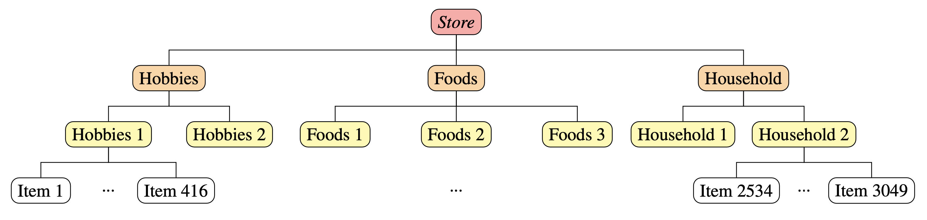
We reproduce the results of the store “CA_1”. The base forecasts (for h=1) of the bottom and upper time series are stored in M5_CA1_basefc available as data in the original ‘bayesRecon’ package in R. The base forecast are computed using ADAM (Svetunkov and Boylan 2023), implemented in the R package smooth (Svetunkov 2023).
import pandas as pd
import numpy as np
import time

M5_CA1_basefc = pd.read_pickle('data/M5_CA1_basefc.pkl')

# Hierarchy composed by 3060 time series: 3049 bottom and 11 upper
n_b = 3049
n_u = 11
n = n_u + n_b

#Load A matrix
A = M5_CA1_basefc['A']

# Load base forecasts
base_fc_upper = M5_CA1_basefc['upper']
base_fc_bottom = M5_CA1_basefc['bottom']

# Initialize a dictionary to store the results
rec_fc = {
    'TD_cond': {}
}
Reconciliation via Top-down conditioning
Top down conditioning (TD-cond; see Zambon et al. (2024), Sect. 4) is a reliable approach for reconciling mixed variables in high dimensions. The algorithm is implemented in the function reconc_td_cond(); it takes the same arguments as reconc_mix_cond() and returns reconciled forecasts in the same format.
N_samples_TD = int(1e4)

start = time.time()

# This will raise a warning if upper samples are discarded
td = reconc_td_cond(A, fc_bottom_4rec, fc_upper_4rec,
                   bottom_in_type="pmf", num_samples=N_samples_TD,
                   return_type="pmf", seed=seed)
#Warning: Only 99.6% of the upper samples are in the support of the
#bottom-up distribution; the others are discarded.
stop = time.time()
The algorithm TD-cond raises a warning regarding the incoherence between the joint bottom-up and the upper base forecasts. We will see that this warning does not impact the performances of TD-cond. An important note to be made here is, R and python uses different sampling schemes even with the same seed. So we might see some minor deviations of the results than the ones presented in R. But as we increase N_samples_TD , it becomes negligible.
rec_fc['TD_cond'] = {
    'bottom': td['bottom_reconciled']['pmf'],
    'upper': td['upper_reconciled']['pmf']
}

TDCond_time = round(stop - start, 2)
print(f"Computational time for TD-cond reconciliation: {TDCond_time} seconds")
#Computational time for TD-cond reconciliation: 10.03 seconds
The computational time required for the TD-cond is 10.03 seconds.
Nonlinear reconciliation of Swiss immigration rate
This section reproduces a part of the results as presented in the arxiv preprint Nonlinear Probabilistic Forecast Reconciliation (Biswas et al. 2026).
In particular, we replicate the reconciliation of the one-step ahead (h=1) forecasts of the Swiss immigration rate obtained from the data of Swiss demographic ratios that we publish in this package.
Data and base forecasts
The data are obtained from the Swiss Federal Statistical Office (FSO) of Switzerland, available through the FSO PX-Web API. Switzerland is subdivided into 26 cantons. For each Canton and for whole Switzerland, we have extracted annual counts of immigration flow, population (as of 1st January) from years 1981 to 2024. These correspond to the demographic components required to construct the immigration-to-population ratio.
The immigration structure is illustrated in the figure below for two cantons among the 26 cantons in Switzerland. Here, $P$, $I$, and $R$ denote the foreign population, the number of immigrants, and the immigration rate, respectively. The superscripts $AG$, $ZH$, and $CH$ refer to the Canton of Aargau, the Canton of Zürich, and Switzerland as a whole.

Thus, there are :
- $54$ free time series corresponding to the Cantonal level counts of $I$ and $P$ (including No indications), and
- $29$ constrained time series comprising the Cantonal and Swiss immigration ratios along with the total counts of $I$ and $P$ for the whole of Switzerland for this dataset.
The base forecasts are already available in the package fitted using Auto ARIMA models.
import time
import pickle
import numpy as np
from pathlib import Path

# ------------------------------------------------------------------
# Load base forecasts and test data
# ------------------------------------------------------------------

forecast_dir = Path("../data")

def load_pickle(filename):
    path = forecast_dir / filename
    with path.open("rb") as f:
        return pickle.load(f)

base = load_pickle("fc_imm_cit_autoarima2_30.pkl")
base_2 = load_pickle("fc_imm_cit_autoarima_30.pkl")
test_data = load_pickle("test_autoarima_30.pkl")
test_data_2 = load_pickle("test_autoarima2_30.pkl")
Nonlinear reconciliation via UKF-based conditioning
Since the structure of the data, and the way the base forecasts were saved is a bit complex we need to define some pre-processing functions before reconciliation.
def f_constrained_from_free(Bns, ref_id):
    """
    Vectorized map f: free -> constrained for BUIS.
    free Bns: (N, 2U) with order [imm(U), pop(U)].
    Returns constrained: (U+1, N) with order [mid_ratios(U), top_ratio(1)].
    where mid_k = imm_k / pop_k, and top = sum_k w_k * mid_k.
    """
    U = Bns.shape[1] // 2
    imm = Bns[:, :U]
    pop = Bns[:, U:]
    mid_total = np.concatenate([np.sum(imm, axis=1, keepdims=True), np.sum(pop, axis=1, keepdims=True)], axis=1)
    no_ind_pos = np.where(np.array(ref_id) == 'No indication')[0].tolist()
    mid_ratio = np.delete(imm, no_ind_pos, axis=1) / (np.delete(pop, no_ind_pos, axis=1) + 1e-8)
    top = np.sum(imm, axis=1, keepdims=True) / np.sum(pop, axis=1, keepdims=True)
    constrained = np.concatenate([top, mid_ratio, mid_total], axis=1)
    return constrained.T

def f_constrained_from_free_single(z, no_ind_pos):
    U = z.shape[0] // 2
    imm = z[:U]
    pop = z[U:]
    mid_total = np.concatenate([np.atleast_1d(np.sum(imm)), np.atleast_1d(np.sum(pop))])
    mid_ratio = np.delete(imm, no_ind_pos) / (np.delete(pop, no_ind_pos) + 1e-8)
    top = np.atleast_1d(np.sum(imm) / np.sum(pop))
    return np.concatenate([top, mid_ratio, mid_total])
Nonlinear reconciliation via UKF-based conditioning (UKF; see Biswas et. al. (2026), Sect. 3.2) is a fast and reliably accurate approach to reconcile continuous base forecasts that can be approximated by a Gaussian distribution. In particular, projection-based approaches needs optimization techniques to project the base forecast samples into the coherent manifold which makes it time-consuming. The UKF however, relies on matrix algebra and thus, is computationally effective and fast.
The algorithm is implemented in the function reconc_nl_ukf that takes the following as input:
-
free base forecasts: a list of $n_b$ dictionaries, each containing "samples" and "residuals" for the free series -
in_type: a list of length $n_b$ indicating the type of each free series (e.g., "samples" or "distr") -
distr: a list of length $n_b$ containing the distribution type for each free series (e.g., "gaussian"); can be empty if in_type is "samples" -
f_u: FTC function -
constrained base forecasts: array of shape (n_u) containing the mean vector of base forecasts for the constrained series -
R: array of shape (n_u, n_u) containing the covariance matrix of the constrained series (estimated from residuals) -
num_samples: number of reconciled samples to generate -
seed: random seed for reproducibility
t0_ukf_imm = time.perf_counter()
nlukf_imm = {}

for t in range(T):
    u_obs = np.mean(np.vstack([imm_ratio_top[:, t, :], imm_ratio_mid[:, t, :],
                                   imm_total[:,t,:], pop_total[:,t,:]]), axis=1)
    R = _schafer_strimmer_cov((np.vstack([imm_ratio_top_res[:, t, :],
                                              imm_ratio_mid_res[:, t, :],
                                              imm_total_res[:,t,:],
                                              pop_total_res[:,t,:]])).T)['shrink_cov']

    free_list = []
    for k in range(U):  # immigration totals
        free_list.append({"samples": imm_free[k, t, :], "residuals": imm_free_res[k, t, :]})
    for k in range(U):  # population totals
        free_list.append({"samples": pop_free[k, t, :], "residuals": pop_free_res[k, t, :]})

    def f_single(z):
        return f_constrained_from_free_single(z, no_ind_pos)

    out = reconc_nl_ukf(
        free_base_forecasts=free_list,
        in_type=["samples"] * (2 * U),
        distr=[] * (2 * U),
        f_u=f_single,
        constrained_base_forecasts=u_obs,
        R=R,
        num_samples=M,
        seed=42,
    )
    Brec = out["free_reconciled_samples"]
    Urec = f_constrained_from_free(Brec.T, ref_id=ref_uids)
    nlukf_imm[t] = np.vstack([Urec, Brec])

nlukf_imm = np.stack([nlukf_imm[t] for t in range(T)], axis=1)
print("Time taken to reconcile:", time.perf_counter() - t0_ukf_imm,"seconds")
# Time taken to reconcile: 1.69 seconds
The computational time required for the UKF is 1.69 seconds.
Contributors


Project details
Verified details
These details have been verified by PyPIProject links
GitHub Statistics
Maintainers
Release history Release notifications | RSS feed


Download files
Download the file for your platform. If you're not sure which to choose, learn more about installing packages.
Source Distribution
Built Distribution
Filter files by name, interpreter, ABI, and platform.
If you're not sure about the file name format, learn more about wheel file names.
Copy a direct link to the current filters
File details
Details for the file bayesreconpy-0.5.0.tar.gz.
File metadata
- Download URL: bayesreconpy-0.5.0.tar.gz
- Upload date:
- Size: 69.7 kB
- Tags: Source
- Uploaded using Trusted Publishing? Yes
- Uploaded via: twine/6.1.0 CPython/3.13.12
File hashes
| Algorithm | Hash digest | |
|---|---|---|
| SHA256 |
d9bcbb8fa8758b4e7c2ad23e047b4e4469be4dfb9418b9965da2a6821c92034a
|
|
| MD5 |
d385df0c157cd6e0fce104eb77df864c
|
|
| BLAKE2b-256 |
38ab905f515a937a82ede545e454456141c5aea227e1a6206af46f2296e800de
|
Provenance
The following attestation bundles were made for bayesreconpy-0.5.0.tar.gz:
Publisher:
pypi-publish.yml on supsi-dacd-isaac/BayesReconPy
-
Statement:
-
Statement type:
https://in-toto.io/Statement/v1 -
Predicate type:
https://docs.pypi.org/attestations/publish/v1 -
Subject name:
bayesreconpy-0.5.0.tar.gz -
Subject digest:
d9bcbb8fa8758b4e7c2ad23e047b4e4469be4dfb9418b9965da2a6821c92034a - Sigstore transparency entry: 1497101115
- Sigstore integration time:
-
Permalink:
supsi-dacd-isaac/BayesReconPy@79cd56febf2bc3e0b21d4f2e705972e04a8723aa -
Branch / Tag:
refs/tags/v0.5.0 - Owner: https://github.com/supsi-dacd-isaac
-
Access:
public
-
Token Issuer:
https://token.actions.githubusercontent.com -
Runner Environment:
github-hosted -
Publication workflow:
pypi-publish.yml@79cd56febf2bc3e0b21d4f2e705972e04a8723aa -
Trigger Event:
push
-
Statement type:
File details
Details for the file bayesreconpy-0.5.0-py3-none-any.whl.
File metadata
- Download URL: bayesreconpy-0.5.0-py3-none-any.whl
- Upload date:
- Size: 83.2 kB
- Tags: Python 3
- Uploaded using Trusted Publishing? Yes
- Uploaded via: twine/6.1.0 CPython/3.13.12
File hashes
| Algorithm | Hash digest | |
|---|---|---|
| SHA256 |
0645b8701181260947adf2f689687fa63cb169719ce91a79ed07872694b1b72e
|
|
| MD5 |
c2cda0b0ed2634ab50a1f3819af54887
|
|
| BLAKE2b-256 |
55609080ecde837518b4f9d70f25b2e344dcb6e0e2f91dbc352feececfbf3cf5
|
Provenance
The following attestation bundles were made for bayesreconpy-0.5.0-py3-none-any.whl:
Publisher:
pypi-publish.yml on supsi-dacd-isaac/BayesReconPy
-
Statement:
-
Statement type:
https://in-toto.io/Statement/v1 -
Predicate type:
https://docs.pypi.org/attestations/publish/v1 -
Subject name:
bayesreconpy-0.5.0-py3-none-any.whl -
Subject digest:
0645b8701181260947adf2f689687fa63cb169719ce91a79ed07872694b1b72e - Sigstore transparency entry: 1497101191
- Sigstore integration time:
-
Permalink:
supsi-dacd-isaac/BayesReconPy@79cd56febf2bc3e0b21d4f2e705972e04a8723aa -
Branch / Tag:
refs/tags/v0.5.0 - Owner: https://github.com/supsi-dacd-isaac
-
Access:
public
-
Token Issuer:
https://token.actions.githubusercontent.com -
Runner Environment:
github-hosted -
Publication workflow:
pypi-publish.yml@79cd56febf2bc3e0b21d4f2e705972e04a8723aa -
Trigger Event:
push
-
Statement type:


