

A package for Bayesian Changepoint detection via Logistic Regression.
These methods were developed in Thomas, Jauch, and Matteson (2025).
Installation
The simplest way to install the package, is to install from PyPI via the code:
pip install bclr
Alternatively, if you would like to install the source code, you can clone the repository and then install via pip (Linux/Mac):
git clone https://github.com/manilasoldier/bclr.git
cd bclr
pip install .
or run
pip install git+https://github.com/manilasoldier/bclr.git
Running the code
import bclr
import numpy as np
np.random.seed(800037)
a1 = np.random.standard_t(10, size=(320, 6))
a2 = np.random.standard_t(1.5, size=(480, 6))

# "Gaussian" type embedding
Xs = np.exp(-np.r_[a1, a2]**2)
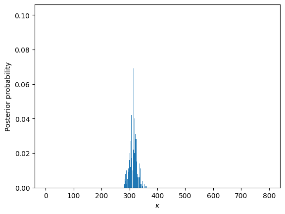
Let's first investigate the single changepoint setup, before moving the multiple one.
First, let's specify a prior for the $\beta$ coefficients (we need to provide a mean and covariance for the single changepoint setup).
Single changepoint setup
rng1 = np.random.default_rng(800037) #for reproducibility
prior_covS = np.diag(np.repeat(3, 6))
prior_mean = np.repeat(0, 6)

bclrS = bclr.BayesCC(X = Xs, prior_mean = prior_mean, prior_cov = prior_covS,
                     n_iter = 2000)
bclrS.fit(rng = rng1)
bclrS.transform(verbose=False)
bclrS.plot_k()
Multiple changepoint setup
Now we consider the multiple changepoint setup and the whole series $X$, where specify $J = 10$ (i.e. cps=10).
Then, we will go ahead and fit bclr to the data and estimate (predict) the changes.
Note: there is no need to specify a prior_mean for the multiple changepoint setup.
np.random.seed(199203)
b1 = np.random.randn(100, 10)
b2 = np.random.randn(80, 10) + np.broadcast_to(np.random.randn(10), (80, 10))
b3 = np.random.randn(140, 10) + np.broadcast_to(np.random.randn(10), (140, 10))
b4 = np.random.randn(80, 10) + np.broadcast_to(np.random.randn(10), (80, 10))

Xm = np.r_[b1, b2, b3, b4]
rng2 = np.random.default_rng(199203) #for reproducibility
prior_covM = np.diag(np.repeat(3, 10))
bclrM = bclr.MultiBayesCC(X = Xm, cps = 10, prior_cov = prior_covM,
                          rng = rng2, warnings=False)
cps = bclrM.fit_predict()
Now we can look at
- where the changes are estimated to be located,
- the posterior probability of the estimates, and
- the normalized entropy of the segment distribution.
print(cps)
   Location  Posterior Probability  Normalized Entropy
0      99.0                  0.946            0.047544
1     180.0                  1.000            0.000000
2     320.0                  0.996            0.005354
1 maintainer

Metadata
1 maintainer
Release files for bclr 0.3.3
For a detailed explanation of source distributions (sdists) and built distributions (wheels), please see the package formats documentation.
Source distribution (sdist)
| File | Size | Uploaded | |
|---|---|---|---|
| bclr-0.3.3.tar.gz | 39.4 kB | Details |
Built distribution (wheel)
| File | Interpreter | ABI | Platform | Reset |
|---|---|---|---|---|
| bclr-0.3.3-py3-none-any.whl | Python 3 | none | any | Details |
Total release size: 73.9 kB
Release files / bclr-0.3.3.tar.gz
| Download URL | bclr-0.3.3.tar.gz |
|---|---|
| Size | 39.4 kB |
| Tags | Source |
|
SHA-256 checksum How to use checksums |
d729fe3e4246079f7a2f261a3e86eae4fa9ef160f0d1465a19b7b80251db374c
|
|
BLAKE2b-256 checksum How to use checksums |
e926e83d8551b5172a885e031de13c28ae0a1cd0374bc99d3dba3662b05fa89a
|
| Upload date | |
|
Uploaded using Trusted Publishing? What is trusted publishing? |
No |
| Uploaded via |
twine/6.1.0 CPython/3.12.0
|
Release files / bclr-0.3.3-py3-none-any.whl
| Download URL | bclr-0.3.3-py3-none-any.whl |
|---|---|
| Size | 34.5 kB |
| Tags | Python 3 |
|
SHA-256 checksum How to use checksums |
5e7fdc9a251dd91d48f4b5b8f0a5308d7c75bb708afba28ac4a878ae41c5bc1d
|
|
BLAKE2b-256 checksum How to use checksums |
e66a808633228260001c4ecf0edb9f2ad3ed4f596317862a0dea4e8e0889e1d7
|
| Upload date | |
|
Uploaded using Trusted Publishing? What is trusted publishing? |
No |
| Uploaded via |
twine/6.1.0 CPython/3.12.0
|














