
BEST
(Batched Emulator Sampling with TensorFlow)
A TensorFlow-based inference framework for high-performance Markov Chain Monte Carlo (MCMC) sampling, profile likelihood optimisation, and nested sampling, including support for neural likelihood emulators, adaptive covariance estimation, and GPU acceleration.
Overview
best is a TensorFlow-based inference framework designed for modern accelerator hardware. All algorithms are implemented using vectorized TensorFlow operations and can be JIT compiled with XLA, enabling efficient execution on GPUs for Bayesian posterior sampling, Bayesian evidence estimation, and profile likelihood optimisation.
Supported MCMC samplers
- Metropolis-Hastings (MH)
- Affine Invariant Ensemble Sampler (AIES)
- Hamiltonian Monte Carlo (HMC)
- No-U-Turn Sampler (NUTS)
- Metropolis Adjusted Langevin Algorithm (MALA)
Key features
- End-to-end TensorFlow implementation
- GPU and XLA compatible throughout
- Batched execution across chains, optimisations and nested-sampling updates
- Automatic covariance estimation during burn-in
- Automatic clustering for multimodal nested sampling
- Covariance-adapted slice sampling
- Posterior reconstruction from weighted dead points
- Neural likelihood emulator support
- Pretrained neural likelihood emulators
Installation
From PyPI
pip install best-inference
From source
git clone https://github.com/AndreasNygaard/best-inference.git
cd best-inference
pip install .
Quick start
Bayesian MCMC sampling
import best
import tensorflow as tf

def log_prob(x):
    return -0.5 * tf.reduce_sum(x**2, axis=-1)

sampler = best.Sampler(log_prob, bounds=([-5, -5], [5, 5]))

results = sampler.sample(
    method="hmc",
    n_steps=2000,
    n_chains=50,
    initial_distribution="uniform",
    num_burnin_steps=1000
)

print(results.samples.shape)
print(results.loglkl.shape)
Frequentist profile likelihoods
import best
import tensorflow as tf

def log_prob(x):
    return -0.5 * tf.reduce_sum(x**2, axis=-1)

optimiser = best.Optimiser(log_prob, bounds=([-5, -5, -5], [5, 5, 5]))

# 2D profile with the first two parameters fixed (0 and 1)
results = optimiser.compute_profile([0,1])

print(results.full_position.shape)
print(results.loglkl.shape)
Nested sampling
import best
import tensorflow as tf
import numpy as np

def log_prob(x):
    return -0.5 * tf.reduce_sum(x**2, axis=-1)

d=3
n_live = 1000
nested_sampler = best.NestedSampler(log_prob, bounds=([-5]*d, [5]*d), n_live=n_live)

results = nested_sampler.run()
print('Target logZ   :', d/2*np.log(2*np.pi)-d*np.log(10))
print('Computed logZ :', results.logZ.numpy(), '±', results.sigma_logZ.numpy())
Sampler API
Initialisation
sampler = best.Sampler(
    log_prob_fn,
    bounds=None,
    enforce_boundaries=True,
    covmat=None,
    initial_state=None,
    n_chains=None,
    initial_distribution=None,
    boundary_penalty_factor=10000
)
optimiser = best.Optimiser(
    log_prob_fn,
    bounds,
    covmat=None,
    loc=None,
    mcmc_temperature=1.0
)
nested_sampler = best.NestedSampler(
    log_prob_fn,
    bounds,
    n_live
    n_live_updates=10,
    n_max_iter=100000,
    max_tree_depth=0,
    min_cluster_size=50,
    cluster_merge_tolerance=0.30,
    cluster_update_interval=100,
    slice_factor=5,
    slice_step_size=5.0,
    slice_global_mixing=0.1,
    tolerance=1e-3,
    batch_sorting=True,
    history_correction=True,
    history_correction_iterations=1,
    history_buffer_size=100,
    seed=42,
    dtype=tf.float32
)
Sampling
results_samp = sampler.sample(
    method="mh" | "aies" | "hmc" | "nuts" | "mala",
    n_steps=1000,
    n_chains=10,
    initial_state=None,
    initial_distribution="repeat" | "uniform" | "gaussian",
    bounds=None,
    covmat=None,
    num_burnin_steps=100,
    num_covmat_updates=None,
    update_initial_state=True,
    update_initial_distribution=True,
    continue_distribution=False,
    sampler_kwargs={},
    burnin_kwargs={},
    get_individual_chains=True,
    jit_compile=True,
    progress_bar=True,
    temperature=1.0,
    verbose=True
)
Optimisation
results_opt = optimiser.compute_profile(
    idxs=[], # indices for fixed parameters
    fixed_points=None,
    nbins=20,
    batch_size=10,
    start_temperature=1.0,
    decay_temperature=0.5,
    min_temperature=1e-2,
    nd_fixed=None,
    optimiser="diag_lm" | "diag_gn" | "diag_bfgs" | "diag_dfp" | "gd" | "gd_ls" | "bfgs",
    opt_kwargs={},
    verbose=True,
    jit_compile=True
)
Nested sampling
results_ns = nested_sampler.run(
    update_interval=10,
    display_param_idx=0,
    output_width=None,
    verbose=True,
    batch_sorting=None,
    history_correction=None,
    history_correction_iterations=None,
    history_buffer_size=None,
    seed=None
)
Output
results_samp.samples
results_samp.loglkl
results_samp.acceptance_rate
results_samp.evaluations

results_samp.burnin_samples
results_samp.burnin_loglkl
results_samp.burnin_acceptance_rates
results_samp.burnin_evaluations
results_samp.covmat_estimate
results_opt.fixed_points
results_opt.loglkl
results_opt.reduced_position
results_opt.full_position
results_opt.idxs
results_ns.logZ
results_ns.sigma_logZ
results_ns.logX
results_ns.KLDivergence
results_ns.n_live
results_ns.live_points
results_ns.live_logL
results_ns.dead_points
results_ns.dead_logL
results_ns.dead_logX
results_ns.log_posterior_weights
results_ns.posterior_weights
Client emulators
BEST includes pretrained neural likelihood emulators for cosmology-inspired inference problems.
Available models
- lcdm
- sterile_neutrino
Load a model
from best.client_emulators import load_model_and_scalers

log_prob_fn, lower_bounds, upper_bounds = load_model_and_scalers("lcdm")
Example: emulator-based inference
import best
from best.client_emulators import load_model_and_scalers

log_prob_fn, lower, upper = load_model_and_scalers("lcdm")

sampler = best.Sampler(log_prob_fn, bounds=(lower, upper))

results = sampler.sample(
    method="aies",
    n_steps=5000,
    n_chains=100,
    initial_distribution="uniform",
    num_burnin_steps=2000,
    num_covmat_updates=1
)
Example: emulator-based profile likelihood
import best
from best.client_emulators import load_model_and_scalers

log_prob_fn, lower, upper = load_model_and_scalers("lcdm")

optimiser = best.Optimiser(log_prob_fn, bounds=(lower, upper))

# 2D profile for omega_b and omega_cdm
results = optimiser.compute_profile(
    idxs=[0,1]
)
Example: emulator-based nested sampling
import best
from best.client_emulators import load_model_and_scalers

log_prob_fn, lower, upper = load_model_and_scalers("lcdm")

nested_sampler = best.NestedSampler(log_prob_fn, bounds=(lower, upper), n_live=1000, n_live_updates=100)

# It takes a few minutes to compile. Run on GPU for faster results
results = nested_sampler.run(update_interval=10)
Supported MCMC algorithms
Metropolis-Hastings (MH)
Random-walk MCMC with optional adaptive covariance scaling.
Affine Invariant Ensemble Sampler (AIES)
Efficient for highly anisotropic or correlated parameter spaces.
Hamiltonian Monte Carlo (HMC)
Gradient-based sampling with leapfrog integration.
No-U-Turn Sampler (NUTS)
Adaptive HMC variant with automatic trajectory length selection.
Metropolis Adjusted Langevin Algorithm (MALA)
Gradient-informed diffusion-based sampler.
Supported optimisation algorithms
Gradient Descent (GD)
Preconditioned first-order optimisation with fixed learning rate and covariance-based parameter scaling.
Gradient Descent with Line Search (GD-LS)
Preconditioned first-order optimisation with Armijo backtracking line search for adaptive step size selection.
Diagonal Davidon–Fletcher–Powell (Diag-DFP)
Diagonal quasi-Newton optimisation using the DFP inverse-Hessian update with independent curvature estimates per parameter.
Diagonal Broyden–Fletcher–Goldfarb–Shanno (Diag-BFGS)
Diagonal quasi-Newton optimisation using the BFGS inverse-Hessian update with efficient per-parameter curvature adaptation.
Broyden–Fletcher–Goldfarb–Shanno (BFGS)
Full quasi-Newton optimisation using batched inverse-Hessian updates to learn parameter correlations and local curvature structure.
Diagonal Gauss-Newton (Diag-GN)
Approximate diagonal Gauss–Newton optimisation with online curvature estimation from gradient-based curvature proxies.
Diagonal Levenberg–Marquardt (Diag-LM)*
Damped diagonal Gauss–Newton optimisation with adaptive curvature regularisation for improved robustness in poorly conditioned or non-linear regions.
*Default
Nested sampling algorithm
best implements a recursive cluster-aware nested sampler using covariance-adapted slice sampling. Live points are recursively partitioned into local clusters, each represented by an independently estimated covariance matrix. Constrained proposals are generated by slice sampling along random directions transformed by the local covariance, allowing efficient exploration of highly anisotropic and multimodal posteriors. Multiple live points are replaced simultaneously, making the algorithm naturally suited for batched GPU execution. Parameters are internally transformed to a common scaled prior space for improved numerical stability. The transformation is applied consistently to the likelihood evaluation and prior volume calculation, leaving Bayesian evidences invariant.
- Posterior expectations can be computed directly from the weighted dead points without requiring additional MCMC sampling.
- results.sigma_logZ is the standard nested-sampling estimate of the uncertainty on logZ.
Performance notes
- GPU acceleration is available for MCMC, optimisation and nested sampling through TensorFlow/XLA.
- JIT compilation (XLA) improves performance for large chains.
- Batched execution exploits thousands of simultaneous likelihood evaluations on modern GPUs.
- Covariance estimation is performed during burn-in when enabled.
- Optimiser for profile likelihoods is initialised with an MCMC for exploring the parameter space.
- Nested sampler updates multiple live points simultaneously.
Example: Multi-sampler comparison
sampler.set_initial_state(initial_state=means, covmat=covmat, initial_distribution="gaussian")
res_aies = sampler.sample(method="aies", n_steps=5000, n_chains=100)
res_hmc  = sampler.sample(method="hmc",  n_steps=5000, n_chains=100)
res_nuts = sampler.sample(method="nuts", n_steps=5000, n_chains=100)
res_mh   = sampler.sample(method="mh",   n_steps=5000, n_chains=100)
res_mala = sampler.sample(method="mala", n_steps=5000, n_chains=100)
Refining profile likelihoods
The optimiser is initialised by running an MCMC sampler in order to explore the parameter space and estimate the covariance matrix and the best-fit point. The points sampled here allow for an automatic selection of relevant points for the 1D and 2D profile likelihoods (as to not waste computational effort on bad points in a grid).
It can, however, happen that a few points fail to optimise properly, and this can be inspected using the plot_profile_1d and plot_profile_2d methods producing plots like these (with 1-sigma, 2-sigma, and 3-sigma contours shown as well):
results = optimiser.compute_profile([0,1])
optimiser.plot_profile_2d(results)
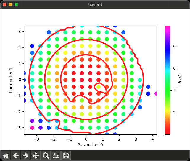
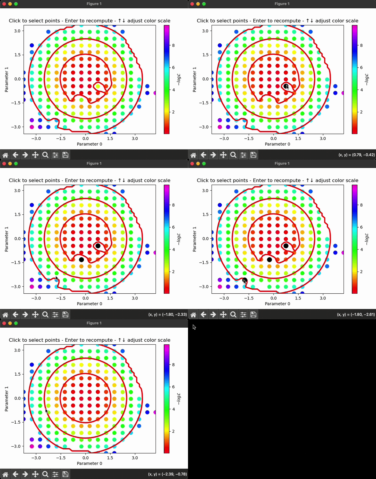
Here, there are three points that stand out (artificially altered for this example), and these can be recomputed using the methods recompute_points_1d and recompute_points_2d. This will open an interactive version of the plot where points can be selected by clicking them and recomputed using the "Enter" key:
updated_results = optimiser.recompute_points_2d(results)
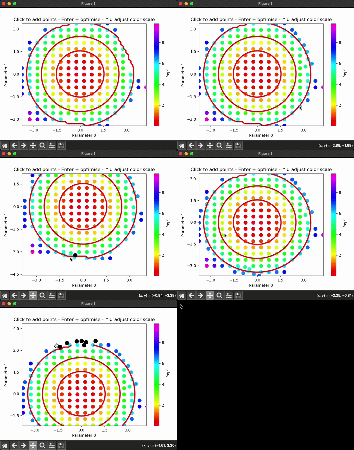
Even though the automatic point selection worked very well, sometimes a few more points are needed to properly represent the 3-sigma contour well enough. In this case, one can use the methods add_points_1d and add_points_2d. This will also open an interactive version of the plot where new points can be added by clicking the desired position and computed using the "Enter" key:
updated_results = optimiser.recompute_points_2d(updated_results)
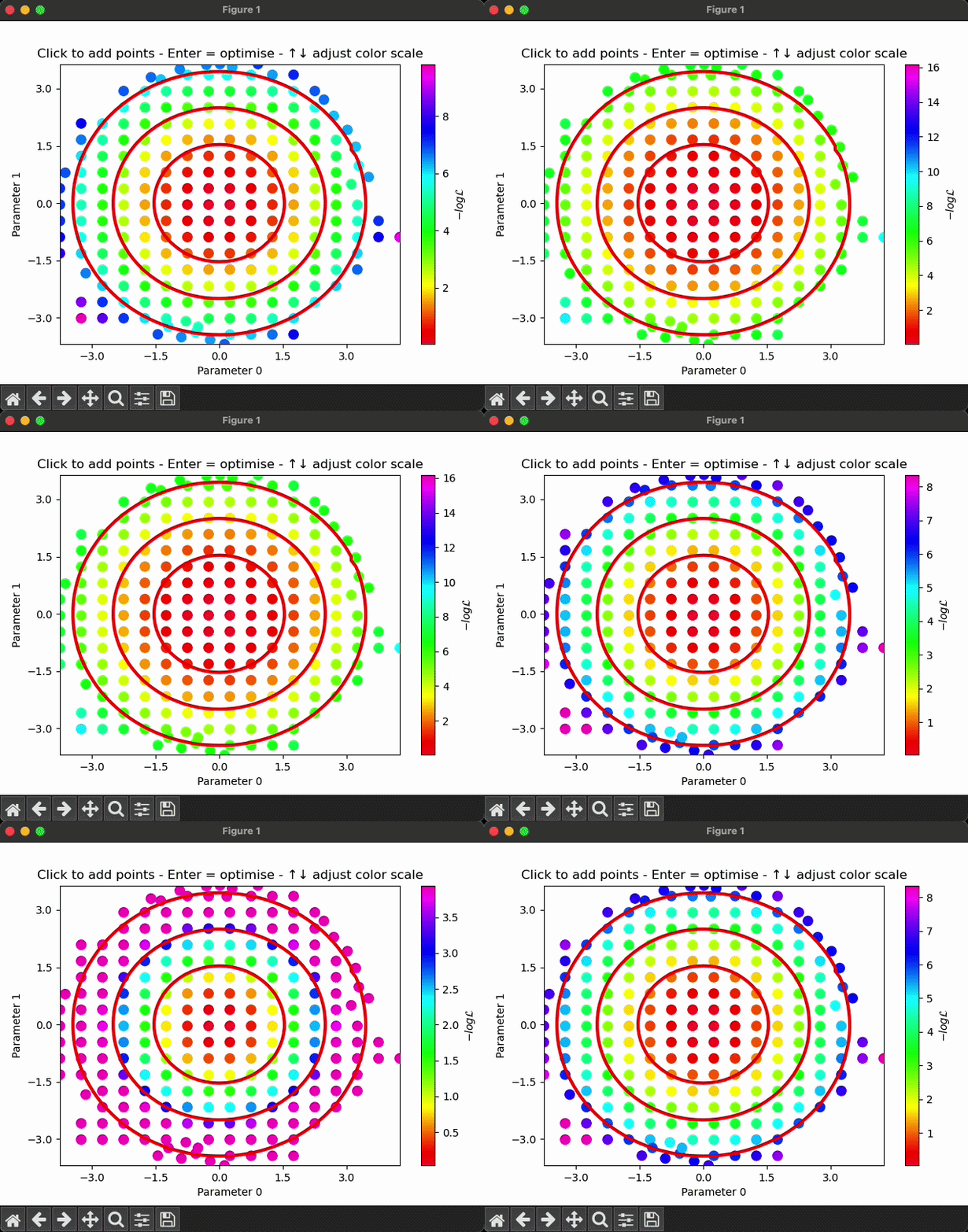
When adding or recomputing points for a 2D profile likelihood, the colour scale can be adjusted using the "up" and "down" arrow keys. This can help better compare adjacent points when the span in likelihood values is quite large:
Nested sampling progress display
When running the nested sampling sampler, a dynamic progress display is shown by default (disable with verbose=False with a faster sampling). An example is shown below:
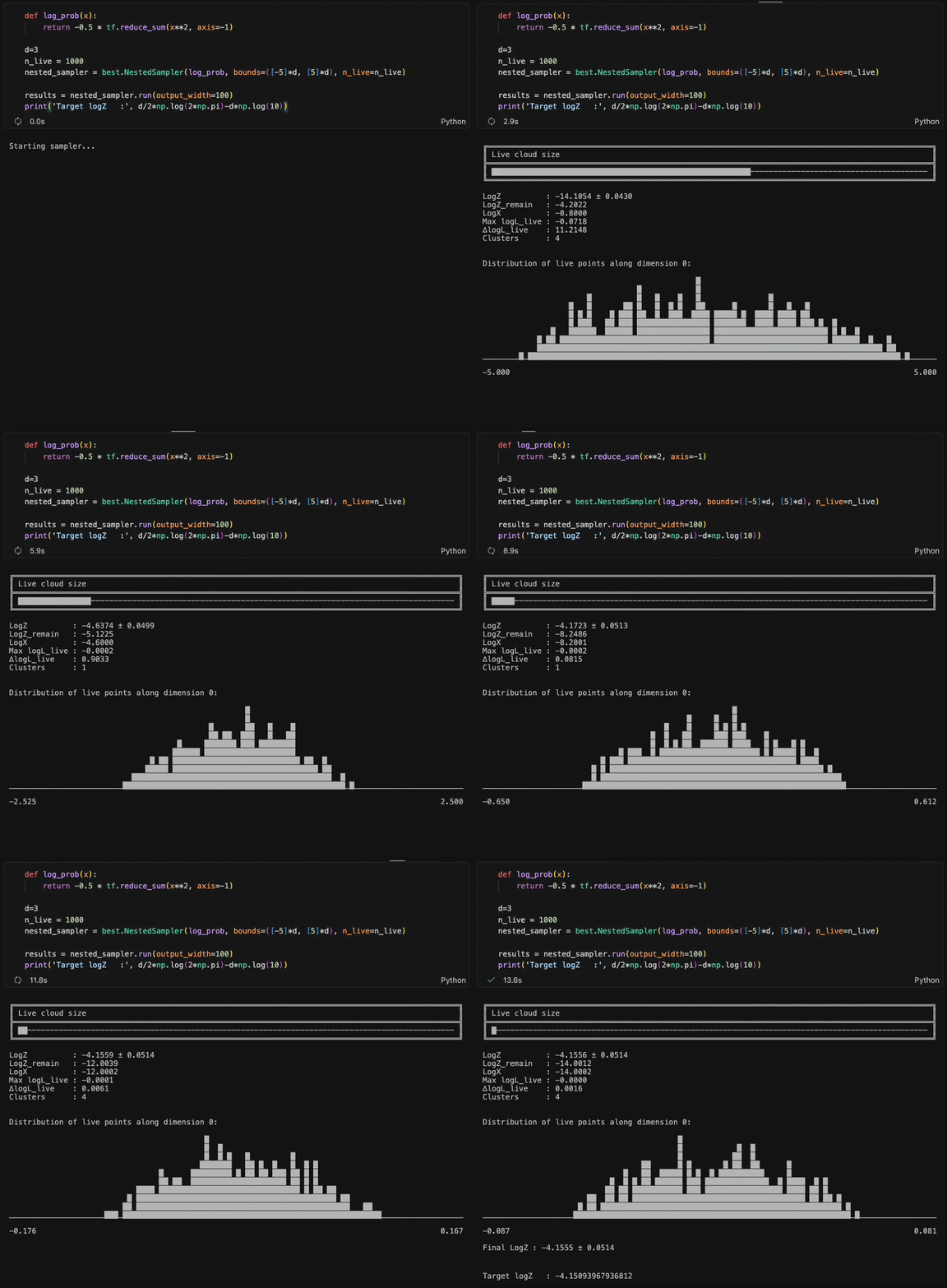
The display provides a real-time overview of the sampling progress and contains:
- A representation of the current live-point cloud size relative to its initial size
- A histogram of the current live points along a selected parameter dimension (chosen with the
display_param_idxkeyword argument) - Current estimates of:
- log-evidence (
logZ) - estimated uncertainty on the log-evidence
- remaining possible log-evidence contribution (
logZ_remain) - log prior volume fraction (
logX) - maximum log-likelihood among live points
- spread in log-likelihood values among live points
- number of detected clusters
- log-evidence (
The sampler terminates automatically when the evidence estimate has converged and is no longer changing significantly. The remaining evidence estimate is shown as an additional diagnostic of the unconstrained contribution from the remaining live points.
For multimodal likelihoods, the evolution of the live-point distribution can be monitored using the histogram display. For example:
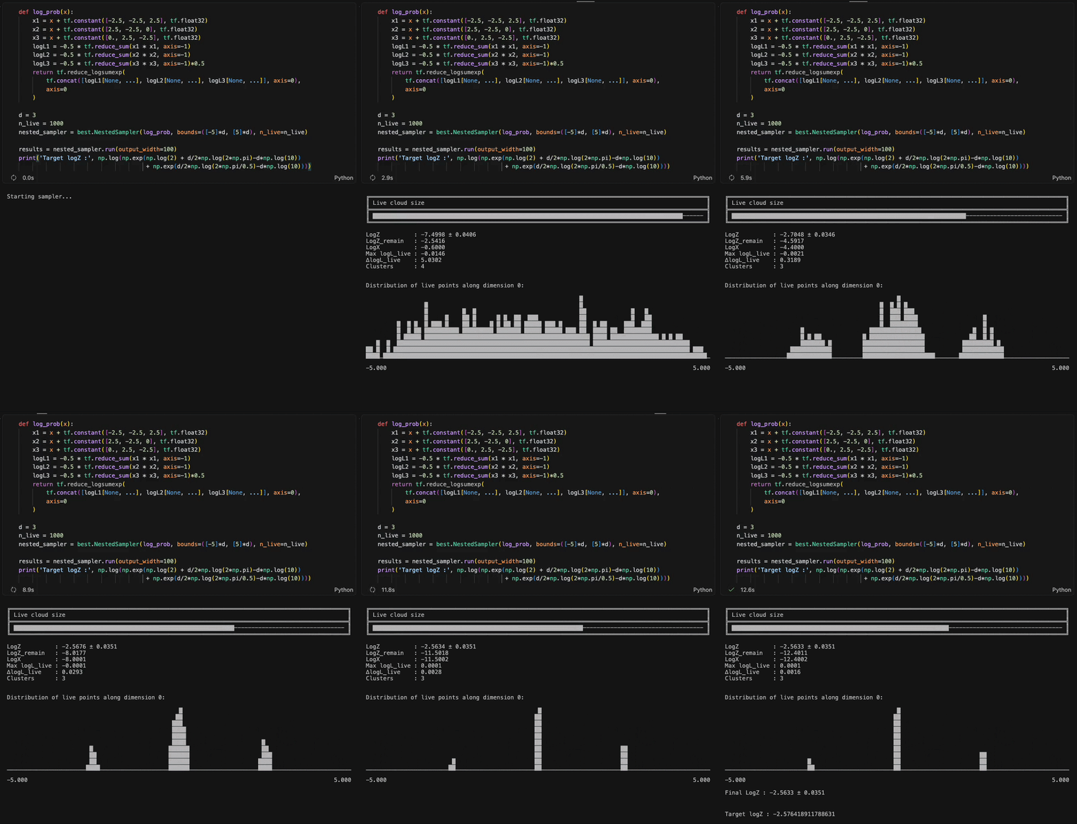
The clustering and live-point diagnostics are intended to provide insight into the behaviour of the sampler, including mode separation, contraction of the live-point cloud, and convergence towards the final evidence estimate.
Requirements
- Python ≥ 3.10
- TensorFlow ≥ 2.17
- TensorFlow Probability ≥ 0.24
- NumPy
- tf-keras
- hypersphere-sampler
Citation
If you use this package, please cite:
@article{Nygaard:2026fgl,
    author = "Nygaard, Andreas and Janken, Luca and Hannestad, Steen and Tram, Thomas",
    title = "{Posterior sampling in the Age of Emulators}",
    eprint = "2606.04895",
    archivePrefix = "arXiv",
    primaryClass = "astro-ph.IM",
    month = "6",
    year = "2026"
}
as well as this one (if using the nested sampler):
@article{Nygaard:2026hbr,
    author = "Nygaard, Andreas",
    title = "{Fast and efficient nested sampling with BEST}",
    eprint = "2608.28514",
    archivePrefix = "arXiv",
    primaryClass = "astro-ph.IM",
    month = "8",
    year = "2026"
}
Contributing
Contributions are welcome. ###Steps:
- Fork repository
- Create feature branch
- Add tests in
tests/ - Submit pull request
License
MIT License
Copyright (c) 2026 Andreas Nygaard
1 maintainer

Release files for best-inference 0.3.4
For a detailed explanation of source distributions (sdists) and built distributions (wheels), please see the package formats documentation.
Source distribution (sdist)
| File | Size | Uploaded | |
|---|---|---|---|
| best_inference-0.3.4.tar.gz | 23.8 MB | Details |
Built distribution (wheel)
| File | Interpreter | ABI | Platform | Reset |
|---|---|---|---|---|
| best_inference-0.3.4-py3-none-any.whl | Python 3 | none | any | Details |
Total release size: 47.6 MB
Release files / best_inference-0.3.4.tar.gz
| Download URL | best_inference-0.3.4.tar.gz |
|---|---|
| Size | 23.8 MB |
| Tags | Source |
|
SHA-256 checksum How to use checksums |
2dfb2efae737b80b73921bd46c97e2b7c5c6a6467ae3574a6d1c0d3671dc46f5
|
|
BLAKE2b-256 checksum How to use checksums |
3b1c42d98e1e4d53b712c56ab1ea63703d1df1774630b51e3ee73eed30a5e149
|
| Upload date | |
|
Uploaded using Trusted Publishing? What is trusted publishing? |
No |
| Uploaded via |
twine/6.2.0 CPython/3.12.2
|
Release files / best_inference-0.3.4-py3-none-any.whl
| Download URL | best_inference-0.3.4-py3-none-any.whl |
|---|---|
| Size | 23.8 MB |
| Tags | Python 3 |
|
SHA-256 checksum How to use checksums |
f5e131f9cfd315200e79a837728d1a5233300bf078905e3d017829efdca04834
|
|
BLAKE2b-256 checksum How to use checksums |
fc323545e9c8acbcafaeef5d48eb401aae6013aebf23836373dfbd99a25ff899
|
| Upload date | |
|
Uploaded using Trusted Publishing? What is trusted publishing? |
No |
| Uploaded via |
twine/6.2.0 CPython/3.12.2
|














