
Boundary effects in spatial graphs: error modeling and untangling strategies
Verified details
These details have been verified by PyPIProject links
GitHub Statistics
Maintainers

Project description
BOSPERRUS: BOundary effects in SPatial graphs: ERRor modeling and Untangling Strategies
Tutorial — Getting Started with Flow
BOSPERRUS detects and corrects boundary effects in spatial graphs. Nodes close to the border of a tissue sample or point cloud tend to have systematically lower centrality scores than nodes in the center — not because they are biologically different, but because they have fewer neighbours. BOSPERRUS models this distance-dependent bias and optionally corrects for it.
Table of Contents
- Installation
- Key concepts
- Quick-start
- Step-by-step walkthrough
- Reading the results
- Choosing a graph type
- Choosing a distance function
- Visualising the correction (optional)
- API reference summary
Installation
Within a conda environment, run
pip install git+https://github.com/bionetslab/bosperrus-package.git
Pip dependencies (scikit-learn, scipy, numpy, pandas) are installed automatically. Within the environment, you also need to
conda install graph-tool -c conda-forge
Key concepts
Entry points / input types:
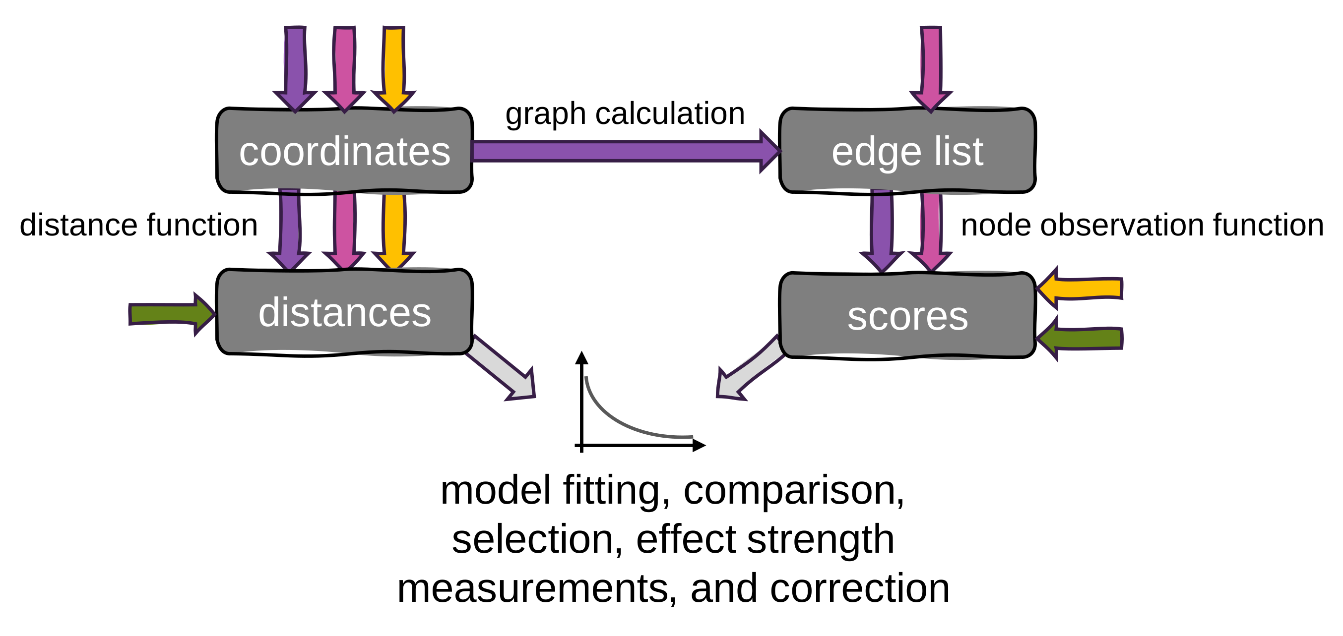
Flow enables multiple entry points depending on what you already have:
🟣 Given coordinates, a distance function, a graph type (Delaunay, k-nearest neighbor, or radius nearest neighbor), and centrality measures to compute.
🩷 Given coordinates, a distance function, and a pre-built edge list.
🟡 Given coordinates, a distance function, and pre-computed centrality scores.
☘️ Given pre-computed distances and scores only (no coordinates needed).
Distance functions:
Quick-start
import numpy as np
from bosperrus import Flow
from bosperrus.distances import distance_to_convex_hull

rng = np.random.default_rng(42)
coords = rng.uniform(0, 100, size=(500, 2))   # 500 random 2-D points

flow = Flow.from_coords(
    coordinates=coords,
    distance_fn=distance_to_convex_hull,
    measures=["degree", "closeness", "betweenness", "clustering", "pagerank"],
    graph_type="delaunay",
)
flow.flow()

# Inspect results
print(flow.fit_quality)
print(flow.observations.head())   # contains raw + corrected centrality columns
Step-by-step walkthrough
Step 1 – Create a toy dataset
We simulate a disc-shaped point cloud to produce an obvious boundary effect: nodes at the perimeter will always have fewer neighbours than nodes at the centre.
import numpy as np
import pandas as pd
import matplotlib.pyplot as plt
from bosperrus import Flow
from bosperrus.distances import distance_to_convex_hull

rng = np.random.default_rng(0)

# Sample uniformly inside a disc of radius 50
n = 600
angles = rng.uniform(0, 2 * np.pi, n)
radii  = 50 * np.sqrt(rng.uniform(0, 1, n))   # sqrt for uniform area sampling
coords = np.stack([radii * np.cos(angles),
                   radii * np.sin(angles)], axis=1)
Step 2 – Initialise Flow
Flow is initialised via one of four factory classmethods depending on what you already have. For a full pipeline from coordinates:
measures = ["degree", "closeness", "betweenness", "harmonic", "clustering", "pagerank"]

flow = Flow.from_coords(
    coordinates=coords,
    distance_fn=distance_to_convex_hull,
    measures=measures,
    graph_type="delaunay",   # or "knn" / "rnn", see below
)
If you already have an edge list, use Flow.from_coords_and_edgelist. If you already have centrality scores, use Flow.from_coords_and_scores. If you have neither coordinates nor a graph, use Flow.from_distances_and_scores.
All factory methods populate flow.observations: a DataFrame with one row per node containing the centrality scores and the distance column.
Step 3 – Run model fitting and correction
from bosperrus.fit import ConstantFit, PiecewiseLinearFit, ExponentialSaturationFit, MichaelisMentenFit

flow.flow(
    measures=measures,
    fits=[ConstantFit, PiecewiseLinearFit, ExponentialSaturationFit, MichaelisMentenFit],
    calculate_rel_ll_to_baseline=ConstantFit,   # ConstantFit = "no boundary effect" null model
)
flow() selects the best model per measure by AIC and writes corrected values back into flow.observations. All arguments are optional — omitting them runs all four models on all measures with ConstantFit as baseline.
After this step:
flow.fit_quality— a DataFrame with one row per measure summarising the best model, AIC-based statistics, effect strength, and half-life.flow.observations— now also contains columns named"BOSPERRUS corrected <measure>"for each centrality.
Reading the results
# Overview table
print(flow.fit_quality.T[[
    "best_fit_type",
    "observed_effect_strength",   # signed relative drop from border to centre
    "observed_half_life",         # distance at which ~50% of the effect has decayed
    "affected samples",           # fraction of nodes still in the boundary-affected zone
]])
observed_effect_strength is defined as (c_border − c_centre) / (c_border + c_centre).
A value close to 0 means negligible boundary bias; a value near ±1 means strong bias.
best_fit_type tells you which model won the AIC comparison:
| Model | Interpretation |
|---|---|
Constant Fit |
No detectable boundary effect |
Piecewise Linear Fit |
Linear drop up to a breakpoint, then flat plateau |
Exponential Saturation Fit |
Smooth exponential approach to a plateau |
Michaelis-Menten Fit |
Hyperbolic saturation (analogous to enzyme kinetics) |
To access the corrected values:
# All corrected columns at once
corrected_cols = [c for c in flow.observations.columns if c.startswith("BOSPERRUS corrected")]
print(flow.observations[corrected_cols].head())

# Single measure
flow.observations[["degree", "BOSPERRUS corrected degree"]].head()
To access fit parameters directly:
degree_fit = flow.best_fits["degree"]
print(degree_fit.name)      # e.g. "Exponential Saturation Fit"
print(degree_fit.params)    # fitted parameter dict
print(degree_fit.AIC)
Choosing a graph type
| Graph type | Key parameter | Notes |
|---|---|---|
"delaunay" |
none | Default choice; produces a natural triangulation without isolated nodes |
"knn" |
k (int) |
Directed, asymmetric — pass via graph_kwargs={"k": 6} |
"rnn" |
r (float, same units as coords) |
Undirected — pass via graph_kwargs={"r": 15.0} |
# k-nearest-neighbour example
flow = Flow.from_coords(
    coordinates=coords,
    distance_fn=distance_to_convex_hull,
    measures=measures,
    graph_type="knn",
    graph_kwargs={"k": 6},
)
Choosing a distance function
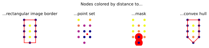
| Function | Use case |
|---|---|
distance_to_convex_hull(coords) |
General default; works for any convex or near-convex tissue shape (2-D and 3-D) |
distance_to_rectangular_border(coords) |
Rectangular imaging window / biopsy (2-D only) |
distance_to_pointset(coords, pointset) |
Border defined by a set of explicit landmark coordinates |
distance_to_mask(coords, mask) |
Binary image mask defining the tissue boundary |
All functions are importable from bosperrus.distances and return a named pd.Series with one value per node.
Visualising the correction (optional)
import matplotlib.pyplot as plt

fig, axes = plt.subplots(1, 2, figsize=(12, 5))

sc = axes[0].scatter(coords[:, 0], coords[:, 1],
                     c=flow.observations["degree"], cmap="viridis", s=8)
axes[0].set_title("Raw degree centrality")
plt.colorbar(sc, ax=axes[0])

sc2 = axes[1].scatter(coords[:, 0], coords[:, 1],
                      c=flow.observations["BOSPERRUS corrected degree"], cmap="viridis", s=8)
axes[1].set_title("BOSPERRUS-corrected degree centrality")
plt.colorbar(sc2, ax=axes[1])

plt.tight_layout()
plt.savefig("bosperrus_correction.png", dpi=150)
plt.show()
Nodes near the border should appear more uniform after correction.
API reference summary
Flow — construction
| Factory method | When to use |
|---|---|
Flow.from_coords(coordinates, distance_fn, measures, graph_type, distance_kwargs=None, graph_kwargs=None) |
Full pipeline from scratch |
Flow.from_coords_and_edgelist(coordinates, distance_fn, measures, edge_list, distance_kwargs=None) |
Skip graph construction |
Flow.from_coords_and_scores(coordinates, distance_fn, scores, distance_kwargs=None) |
Pre-computed centralities |
Flow.from_distances_and_scores(distances, scores) |
No coords needed |
Flow — methods
| Method | Signature | Description |
|---|---|---|
flow |
(measures=None, fits=None, calculate_rel_ll_to_baseline=None) |
Fit all models, select best by AIC, write corrected columns to observations |
Key attributes after a full run
| Attribute | Type | Content |
|---|---|---|
flow.observations |
pd.DataFrame |
All node-level data: centralities, distance column, corrected values |
flow.fit_quality |
pd.DataFrame |
Per-measure model selection summary (columns = measures) |
flow.best_fits |
dict[str, Fit] |
Best Fit object per measure |
flow._edge_list |
set |
Set of edges built during construction (available for Paths 1 and 2) |
Project details
Verified details
These details have been verified by PyPIProject links
GitHub Statistics
Maintainers


Download files
Download the file for your platform. If you're not sure which to choose, learn more about installing packages.
Source Distribution
Built Distribution
Filter files by name, interpreter, ABI, and platform.
If you're not sure about the file name format, learn more about wheel file names.
Copy a direct link to the current filters
File details
Details for the file bosperrus-0.2.0.tar.gz.
File metadata
- Download URL: bosperrus-0.2.0.tar.gz
- Upload date:
- Size: 45.3 kB
- Tags: Source
- Uploaded using Trusted Publishing? Yes
- Uploaded via: twine/6.1.0 CPython/3.13.14
File hashes
| Algorithm | Hash digest | |
|---|---|---|
| SHA256 |
16a37c07b76767fefb8dc6bd5ae3e270cccbd3409e9d9ad0930cebe5afac88ba
|
|
| MD5 |
8f93f1b589d457357e5eb34f7c3b3238
|
|
| BLAKE2b-256 |
eca0b57e80e9ad05923009dcbb06e90f05ddd09807722d0b097302908b6f81ae
|
Provenance
The following attestation bundles were made for bosperrus-0.2.0.tar.gz:
Publisher:
publish.yml on bionetslab/bosperrus-package
-
Statement:
-
Statement type:
https://in-toto.io/Statement/v1 -
Predicate type:
https://docs.pypi.org/attestations/publish/v1 -
Subject name:
bosperrus-0.2.0.tar.gz -
Subject digest:
16a37c07b76767fefb8dc6bd5ae3e270cccbd3409e9d9ad0930cebe5afac88ba - Sigstore transparency entry: 2271351358
- Sigstore integration time:
-
Permalink:
bionetslab/bosperrus-package@b2b9a9d1505ff3bb13ba031238fe3b19b693570e -
Branch / Tag:
refs/tags/v0.2.0 - Owner: https://github.com/bionetslab
-
Access:
public
-
Token Issuer:
https://token.actions.githubusercontent.com -
Runner Environment:
github-hosted -
Publication workflow:
publish.yml@b2b9a9d1505ff3bb13ba031238fe3b19b693570e -
Trigger Event:
release
-
Statement type:
File details
Details for the file bosperrus-0.2.0-py3-none-any.whl.
File metadata
- Download URL: bosperrus-0.2.0-py3-none-any.whl
- Upload date:
- Size: 20.0 kB
- Tags: Python 3
- Uploaded using Trusted Publishing? Yes
- Uploaded via: twine/6.1.0 CPython/3.13.14
File hashes
| Algorithm | Hash digest | |
|---|---|---|
| SHA256 |
e11c250a2e0a6731ab25f73321bd7438e7b873093819403de4d945cf6e02dbec
|
|
| MD5 |
b16a7dae3b8ef5cbae50aa18e28ecb0f
|
|
| BLAKE2b-256 |
a3e995f59536c6df0864e926603a318a36cf8282cc5d23889e39b281ebbf5414
|
Provenance
The following attestation bundles were made for bosperrus-0.2.0-py3-none-any.whl:
Publisher:
publish.yml on bionetslab/bosperrus-package
-
Statement:
-
Statement type:
https://in-toto.io/Statement/v1 -
Predicate type:
https://docs.pypi.org/attestations/publish/v1 -
Subject name:
bosperrus-0.2.0-py3-none-any.whl -
Subject digest:
e11c250a2e0a6731ab25f73321bd7438e7b873093819403de4d945cf6e02dbec - Sigstore transparency entry: 2271351475
- Sigstore integration time:
-
Permalink:
bionetslab/bosperrus-package@b2b9a9d1505ff3bb13ba031238fe3b19b693570e -
Branch / Tag:
refs/tags/v0.2.0 - Owner: https://github.com/bionetslab
-
Access:
public
-
Token Issuer:
https://token.actions.githubusercontent.com -
Runner Environment:
github-hosted -
Publication workflow:
publish.yml@b2b9a9d1505ff3bb13ba031238fe3b19b693570e -
Trigger Event:
release
-
Statement type:






