



Table of contents
BSXplorer
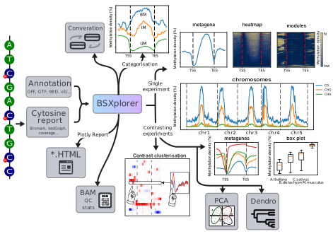
Analytical framework for BS-seq data comparison and visualization. BSXplorer facilitates efficient methylation data mining, contrasting and visualization, making it an easy-to-use package that is highly useful for epigenetic research.
For Python API reference manual and tutorials visit: https://shitohana.github.io/BSXplorer.
How to cite
How to cite
If you use our package in your research, please consider citing our paper.
Yuditskiy, K., Bezdvornykh, I., Kazantseva, A. et al. BSXplorer: analytical framework for exploratory analysis of BS-seq data. BMC Bioinformatics 25, 96 (2024). https://doi.org/10.1186/s12859-024-05722-9
Installation
To install latest stable version:
pip install bsxplorer
If you want to install the prerelease version (dev branch):
pip install pip install git+https://github.com/shitohana/BSXplorer.git@dev
Usage
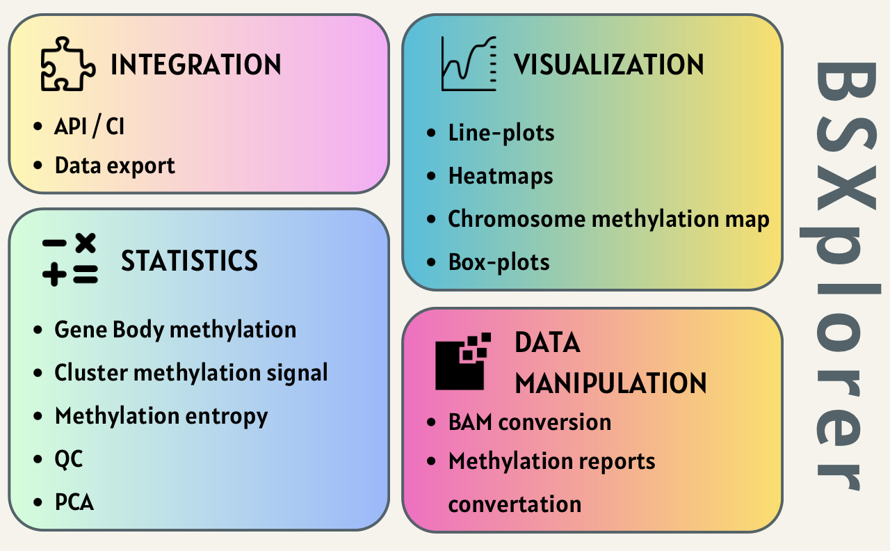
In this project our aim was to create a both powerful and flexible tool to facilitate exploratory data analysis of BS-Seq data obtained in non-model organisms (BSXplorer works for model organisms as well). That's why BSXplorer is implemented as a Python package. Modular structure of BSXplorer together with easy to use and configurable API makes it a highly integratable and scalable package for a wide range of applications in bioinformatical projects.
Even though BSXplorer is available as console application, to fully utilize its potential consider using it as a python package. Detailed documentation can be found here.
API usage
import bsxplorer as bsx
Basic usage
The main objects in BSXplorer are the Genome and Metagene, MetageneFiles
classes. Genome class is used for reading and filtering genomic annotation data.
genome = bsx.Genome.from_gff("path/to/annotation.gff")
Even though here genome was created with .from_gff constructor, to read custom
annotation format (TSV file), use .from_custom and specify column indexes (0-based).
Once we have read annotation file, methylation report can be processed via Metagene
class (or MetageneFiles for multiple reports).
metagene = bsx.Metagene.from_bismark(
    "path/to/report.txt",
    genome=genome.gene_body(min_length=0, flank_length=2000),
    up_windows=100, body_windows=200, down_windows=100
)
Here we have read methylation report file. Methylation data has been read only
for gene bodies (genome.gene_body(min_length=0, flank_length=2000)) with
200 windows resolution for gene body (body_windows=200) and 100 for flanking
regions (up_windows=100, down_windows=100).
Now we can generate visualiztions.
filtered = metagene.filter(context="CG")
filtered.line_plot().draw_mpl()
filtered.heat_map().draw_mpl()
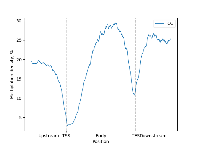
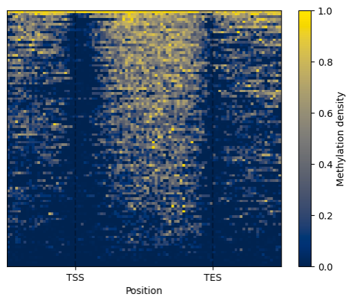
BSXplorer can generate plots with two plotting libraries: matplotlib and Plotly.
_mpl in methods names stands for matplotlib and _plotly for Plotly.
Clusterisation
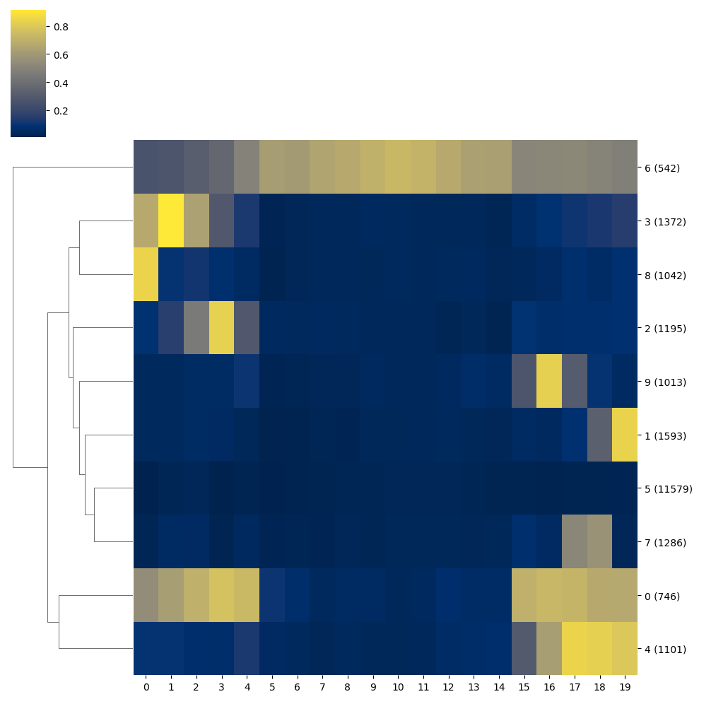
BSXplorer allows for discovery of gene modules characterised with similar methylation patterns.
Once the data was filtered based on methylation context and strand,
one can use the .cluster() method. The resulting object contains an
ordered list of clustered genes and their visualisation in a form of a heatmap.
Chromosome methylation levels
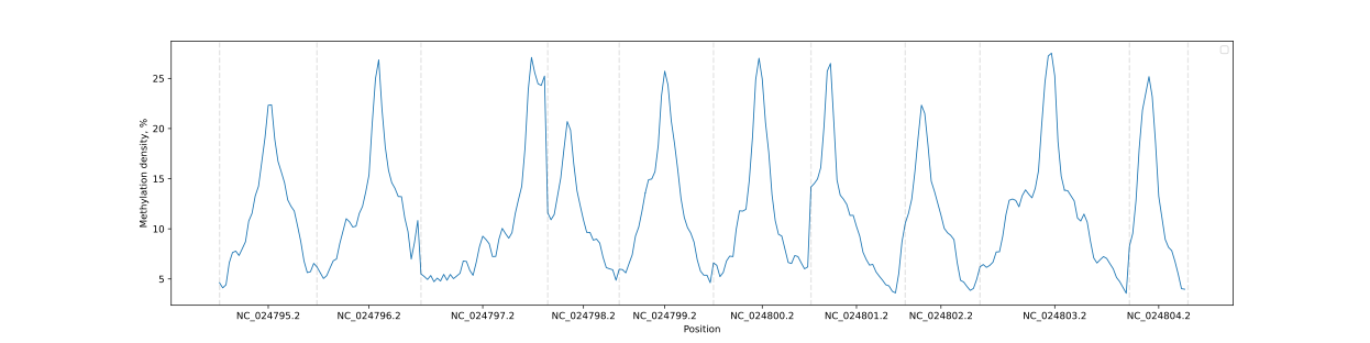
BSXplorer allows a user to visualize the overall methylation levels of chromosomes using the corresponding ChrLevels object:
levels = bsx.ChrLevels.from_bismark("path/to/report.txt", chr_min_length=10**6, window_length=10**6)
levels.draw_mpl(smooth=5)
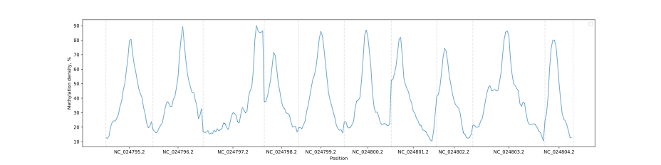
In a way that is similar to the Metagene method, the methylation data can be subjected to filtering to selectively display a methylation context that is of interest.
levels.filter(context="CG").draw_mpl(smooth=5)
Gene body methylation
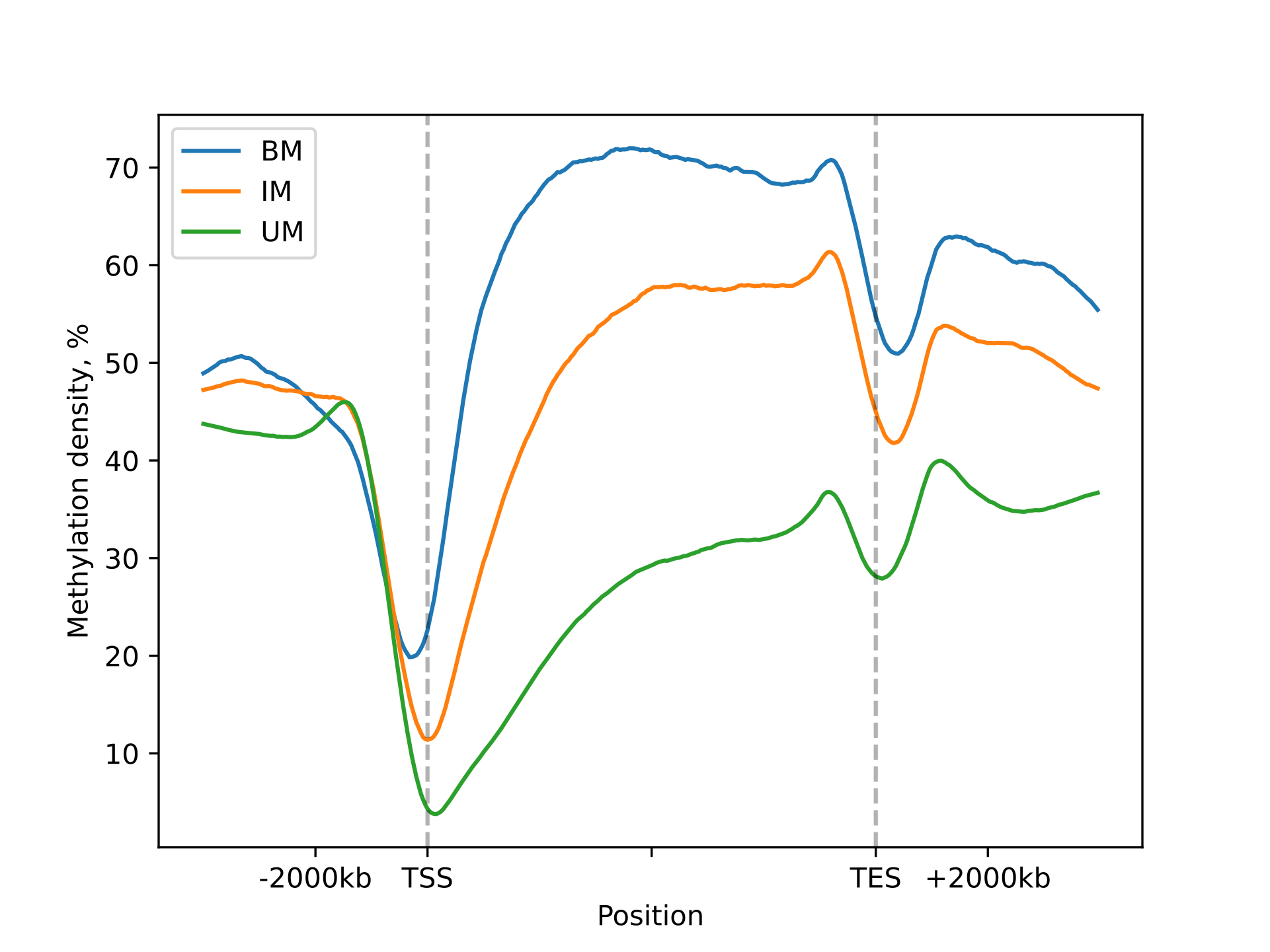
BSXplorer allows for the categorization of regions based on their methylation level and density. This is done by assuming that cytosine methylation levels follow a binomial distribution, as explained in Takuno and Gaut's research (please refer to [1, 2] https://doi.org/10.1073/pnas.1215380110 for details). The genes are then divided into three categories, BM (body-methylated), IM (intermediately-methylated) and UM (under-methylated), based on their methylation levels in the CG context using the following formula.
$$ CG<P_{CG};\ \ CHG/CHH>1-P_{CG} $$
$$ P_{CG}\le CG<1-P_{CG};\ \ CHG/CHH>1-P_{CG} $$
$$ CG/CHG/CHH>1-P_{CG} $$
The same rationale may be applied to other methylation contexts, as BSXplorer can produce $P_{CHG}$ and $P_{CHH}$ for CHG sites and CHH sites, respectively.
[1] Takuno S, Gaut BS. Body-Methylated Genes in Arabidopsis thaliana Are Functionally Important and Evolve Slowly. Mol Biol Evol. 2012;29:219–27.
[2] Takuno S, Gaut BS. Gene body methylation is conserved between plant orthologs and is of evolutionary consequence. Proc Natl Acad Sci. 2013;110:1797–802.
# Calculate pvalue for cytosine methylation via binomial test
binom_data = bsx.BinomialData.from_report(
    "path/to/report.txt",
    report_type="bismark"
)

# Created binomial data object can now be used to calculate pvalues
# for methylation of genomic regions
region_stats = binom_data.region_pvalue(genome.gene_body(), methylation_pvalue=.01)
# .categorise method returns tuple of three DataFrames
# for BM, IM and UM genes respectively
bm, im, um = region_stats.categorise(context="CG", p_value=.05)

# Now we can create MetageneFiles object to visualize methylation pattern
# of categorised groups
cat_metagene = bsx.MetageneFiles([
    metagene.filter(context="CG", genome=bm),
    metagene.filter(context="CG", genome=im),
    metagene.filter(context="CG", genome=um),
], labels=["BM", "IM", "UM"])

# And plot it
tick_labels = ["-2000kb", "TSS", "", "TES", "+2000kb"]
cat_metagene.line_plot().draw_mpl(tick_labels=tick_labels)
Different organisms analysis
Start with import of genome annotation data for species of interest.
arath_genes = bsxplorer.Genome.from_gff("arath_genome.gff").gene_body(min_length=0)
bradi_genes = bsxplorer.Genome.from_gff("bradi_genome.gff").gene_body(min_length=0)
mouse_genes = bsxplorer.Genome.from_gff("musmu_genome.gff").gene_body(min_length=0)
Next, read in cytosine reports for each sample separately:
window_kwargs = dict(up_windows=200, body_windows=400, down_windows=200)

arath_metagene = bsx.Metagene.from_bismark("arath_example.txt", arath_genes, **window_kwargs)
bradi_metagene = bsx.Metagene.from_bismark("bradi_example.txt", bradi_genes, **window_kwargs)
musmu_metagene = bsx.Metagene.from_bismark("musmu_example.txt", mouse_genes, **window_kwargs)
To perform comparative analysis, initialize the bsxplorer.MetageneFiles
class using metagene data in a vector format, where labels for every organism
are provided explicitly.
Next, apply methylation context and strand filters to the input files:
filtered = files.filter("CG", "+")
Then, a compendium of line plots to guide a comparative analyses of methylation patterns in different species is constructed:
filtered.line_plot(smooth=50).draw_mpl()
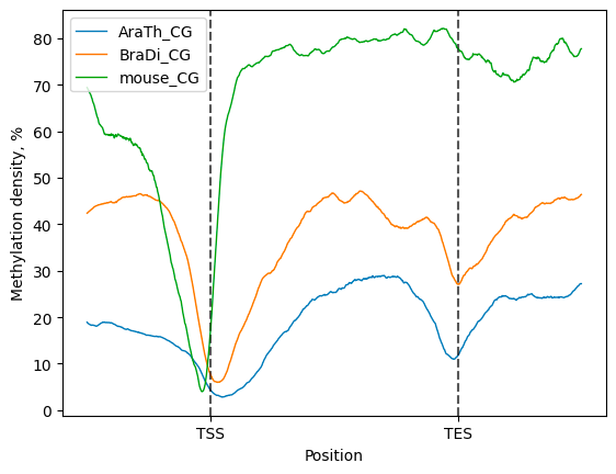
The line plot representation may be further supplemented by a heatmap:
filtered.heat_map(100, 100).draw_mpl()
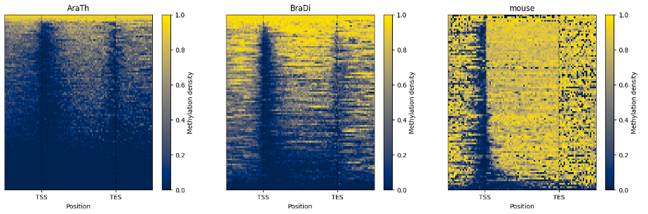
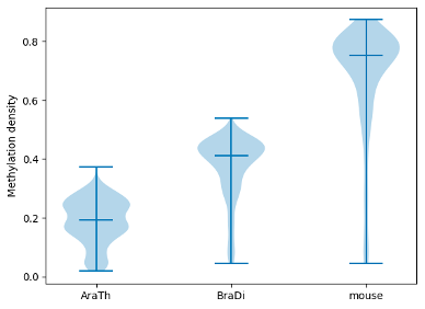
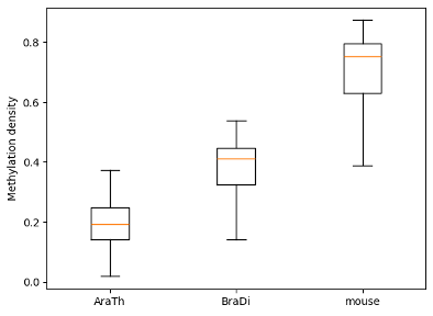
To examine and highlight differences in methylation patterns between different organisms, summary statistics is made available in a graphical format.
filtered.box_plot(violin=True).draw_mpl()
filtered.box_plot().draw_mpl()
Enrichment of DMRs
BSXplorer offers functionality to align one set of regions over another. Regions can
be read either with :class:Genome or initialized directly with
polars functionality <https://docs.pola.rs/api/python/stable/reference/api/polars.read_csv.html>_
(DataFrame need to have chr, start and end columns).
To align regions (e.g. define DMR position relative to genes) or perform the enrichment of regions at these
genomic features against the genome background use :class:Enrichment.
# If you want to perform an ENRICHMENT, and not only plot
# the density of metagene coverage, you NEED to use .raw() method
# for genome DataFrame.
genes = bsx.Genome.from_gff("path/to/annot.gff").raw()
dmr = bsx.Genome.from_custom(
    "path/to/dmr.txt",
    chr_col=0, # Theese columns indexes are configurable
    start_col=1,
    end_col=2
).all()

enrichment = bsx.Enrichment(dmr, genes, flank_length=2000).enrich()
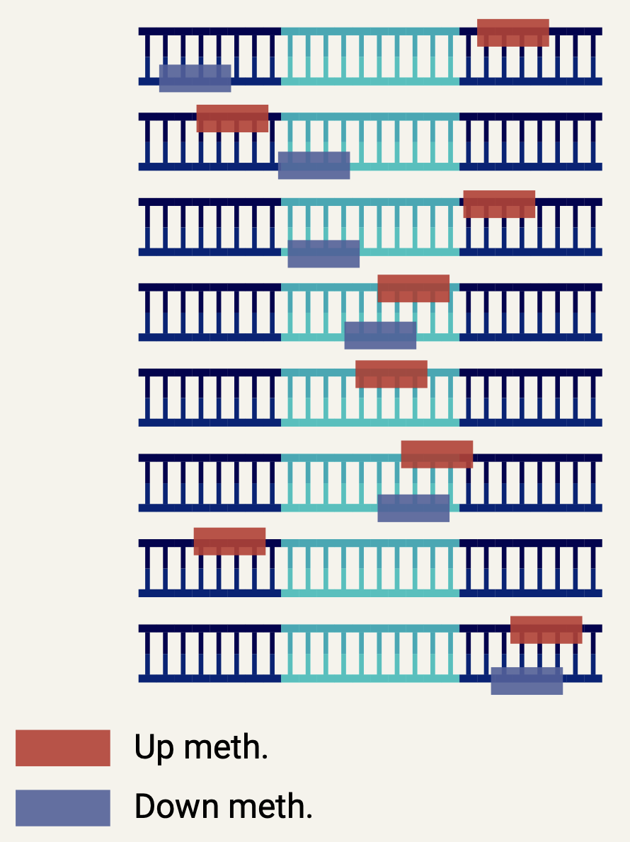
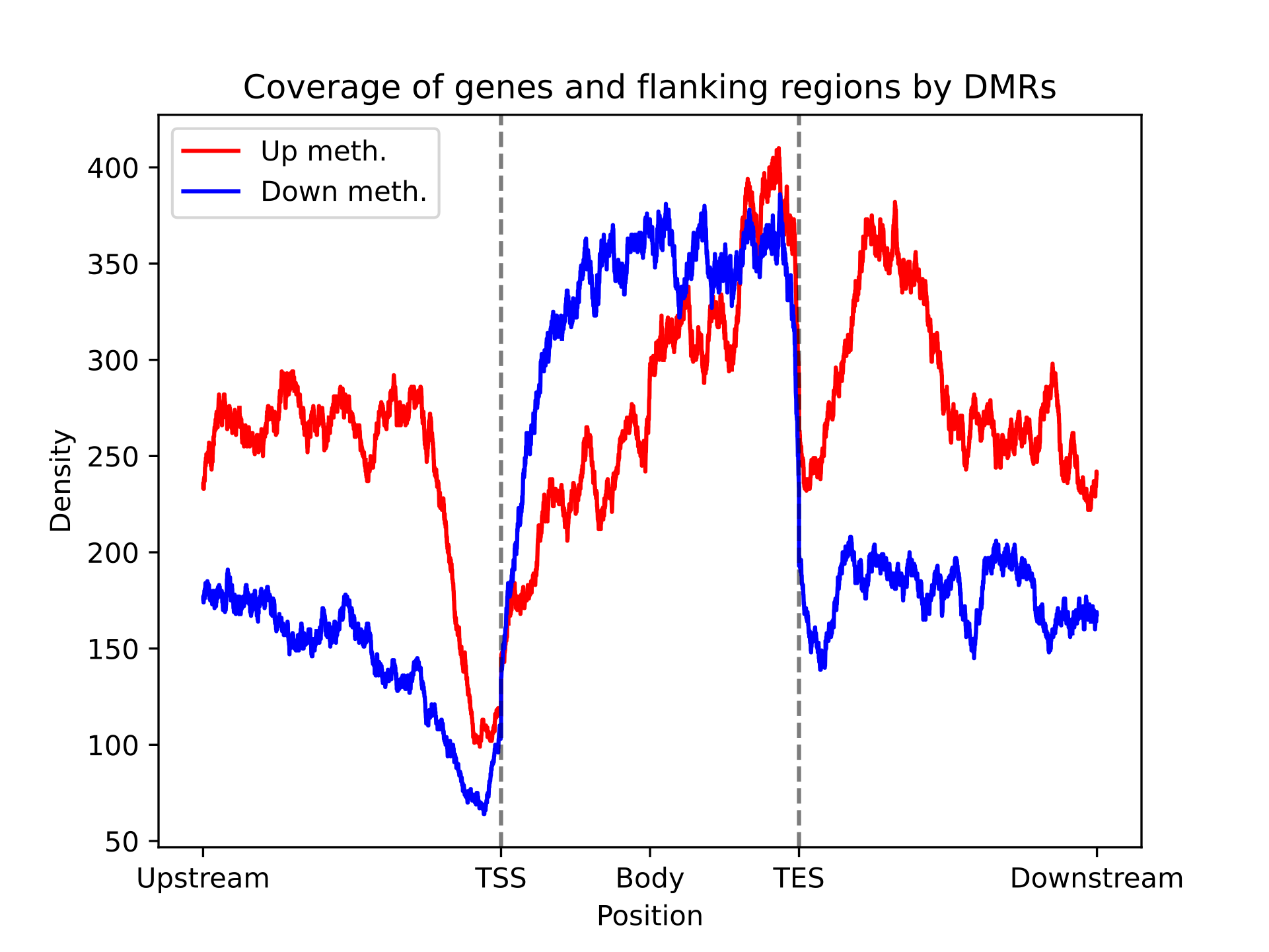
Enrichment.enrich returns EnrichmentResult, which stores enrichment
statistics and coordinates of regions which have aligned with
genomic features. The metagene coverage with regions
can be plotted via EnrichmentResult.plot_density_mpl method.
fig = enrichment.plot_density_mpl(
    tick_labels=["-2000bp", "TSS", "Gene body", "TES" "+2000bp"],
)
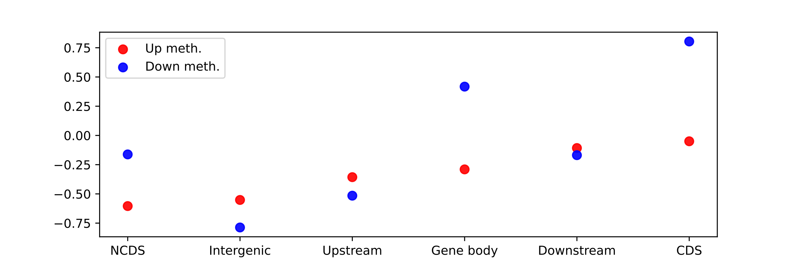
Enrichment statistics can be accessed with EnrichmentResult.enrich_stats
or plotted with EnrichmentResult.plot_enrich_mpl
enrichment.plot_enrich_mpl()
Other functionality
For other functionality, such as methylation reports conversion and BAM conversion and statistics please refer to the documentation.
Console usage
BSXplorer can be used in a console mode for generating complex HTML-reports (see example here) and running many analysis at once or converting BAM to methylation report. For detailed commands description and examples, please refer to the documentation.
What's new
Since publication we have released Version 1.1.0.
Major changes
-
Added new classes for Unified reading of methylation reports (
UniversalReader,UniversalReplicatesReader). Now any supported report type can be converted into another. -
Added support for processing BAM files (
BAMReader). BAM files can be either converted to methylation report (faster than with native methods), or methylation statistics, such as methylation entropy, epipolymorphism or PDR can be calculated. -
Added method for aligning one set of regions along another (e.g. DMR along genes) –
Enrichment. Regions can not only be aligned, but the coverage of the metagene by DMRs can be visualized.
Other improvements
- Any plot data now can be retrieved by corresponding method.
- Fixes to the plotting API.
- Fixes to
Categoryreport. - Added console command for processing BAM files.
1 maintainer

Metadata
1 maintainer
Release files for bsxplorer 1.1.0.post3
For a detailed explanation of source distributions (sdists) and built distributions (wheels), please see the package formats documentation.
Source distribution (sdist)
| File | Size | Uploaded | |
|---|---|---|---|
| bsxplorer-1.1.0.post3.tar.gz | 72.5 kB | Details |
Built distribution (wheel)
| File | Interpreter | ABI | Platform | Reset |
|---|---|---|---|---|
| bsxplorer-1.1.0.post3-py3-none-any.whl | Python 3 | none | any | Details |
Total release size: 152.8 kB
Release files / bsxplorer-1.1.0.post3.tar.gz
| Download URL | bsxplorer-1.1.0.post3.tar.gz |
|---|---|
| Size | 72.5 kB |
| Tags | Source |
|
SHA-256 checksum How to use checksums |
ce85ee8f32bef3a3465343b502d14a828ba0cf22b5ff8d959a2d8d8f86e89032
|
|
BLAKE2b-256 checksum How to use checksums |
52a3e07b3b4944cb2e152ec5399eb2ed8d1d79422712fdb6a4eef4486500ce9c
|
| Upload date | |
|
Uploaded using Trusted Publishing? What is trusted publishing? |
No |
| Uploaded via |
twine/6.1.0 CPython/3.13.12
|
Release files / bsxplorer-1.1.0.post3-py3-none-any.whl
| Download URL | bsxplorer-1.1.0.post3-py3-none-any.whl |
|---|---|
| Size | 80.3 kB |
| Tags | Python 3 |
|
SHA-256 checksum How to use checksums |
c0198818ee7af0d5168d0911c22e18738b98d5bb981affd7911e7c1115ace17d
|
|
BLAKE2b-256 checksum How to use checksums |
069aa479341df8e1033b7dd58e0569e97515b78fa10d2e4e982024073db45e11
|
| Upload date | |
|
Uploaded using Trusted Publishing? What is trusted publishing? |
No |
| Uploaded via |
twine/6.1.0 CPython/3.13.12
|














