
bxai

Bayesian Feature Selection and Attribution Suite
A Python package implementing rigorous Bayesian methods for feature selection and model explainability. Where conjugate structure permits, bxai uses closed-form analytical updates (Beta-Binomial, Normal-Inverse-Gamma) to keep iteration fast. Where the model demands full posterior inference — Horseshoe GLMs, BART, and the optional MCMC path in BayLIME; it delegates to PyMC. The result is a unified toolkit that matches computational cost to statistical necessity.
Features
-
Global Non-Linear Selection
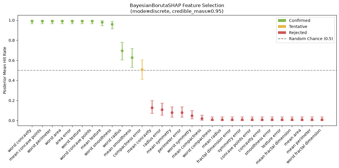
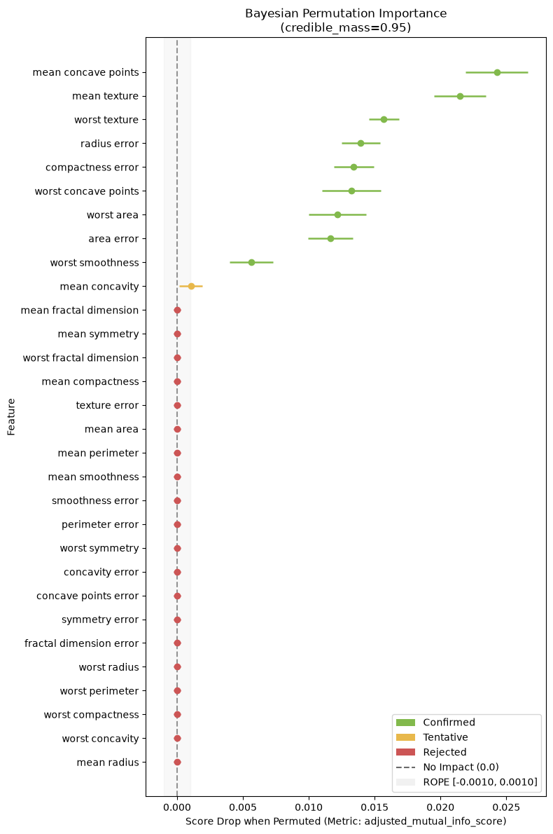
BayesianBorutaSHAP: Tree-based feature selection using SHAP values, swapping frequentist p-values for Bayesian credible intervals, with dynamic pruning for fast performance. Supports discrete (Beta-Binomial) and continuous (Normal-Inverse-Gamma) modes.BayesianPermutation: Model-agnostic importance tracking using paired validation loss drops updated via the Student-t continuous engine.
-
Local Interpretability
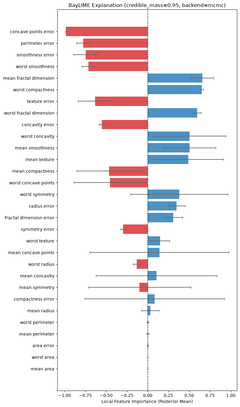
BayLIME: Stable, prior-informed local explanations wrapping standard/custom perturbations in a Bayesian linear regression. The default backend uses a closed-form analytical posterior; an optionalbackend='mcmc'path (requiresmcmcextra) adds heteroscedastic noise and Horseshoe priors for richer uncertainty quantification. Can be seeded with global SHAP weights from Phase 1.
-
Parametric & Native Bayesian Importance
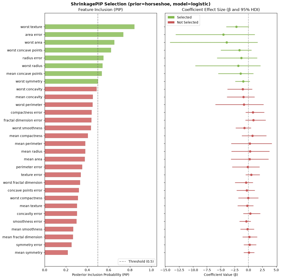
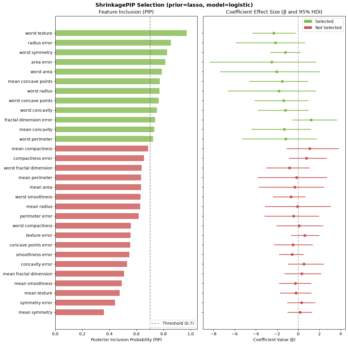
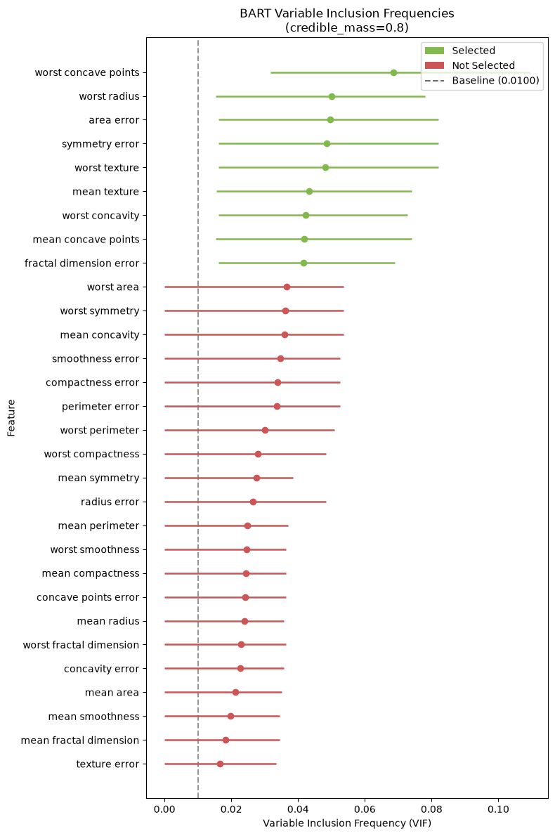
ShrinkagePIP: High-dimensional GLMs with Horseshoe and Lasso regularizing priors, tracking Posterior Inclusion Probabilities (PIP). Uses the posterior shrinkage factor κ_j = 1/(1+λ_j²τ²) for the Horseshoe prior (correct for continuous shrinkage distributions) and an auto-data-scaled |β_j| threshold for the Lasso (requiresmcmcextra).BARTImportance: Variable inclusion frequency (VIF) tracking from native Bayesian Additive Regression Trees (requiresmcmcextra).
Installation
Install using uv:
uv add bxai
Or install with optional dependencies (e.g., SHAP/LightGBM for Boruta, PyMC for MCMC methods, catboost, xgboost):
uv add bxai --optional boruta --optional mcmc --optional xgboost --optional catboost
Quick Start
We will load the real-world Breast Cancer Wisconsin (Diagnostic) dataset as our dataset of choice:
from sklearn.datasets import load_breast_cancer

data = load_breast_cancer(as_frame=True)
X, y = data.data, data.target
BayesianBorutaSHAP
import lightgbm as lgb
from bxai.selection import BayesianBorutaSHAP

# Fit Bayesian BorutaSHAP
clf = lgb.LGBMClassifier(random_state=42, verbose=-1)
selector = BayesianBorutaSHAP(model=clf, mode="discrete", max_iter=20, random_state=42)
selector.fit(X, y)

print("Confirmed Features:", selector.confirmed_)
BayesianPermutation
from bxai.selection import BayesianPermutation
from sklearn.ensemble import RandomForestClassifier

clf_perm = RandomForestClassifier(random_state=42).fit(X, y)

# Permutation feature selection with parallel jobs (n_jobs=2) and ROPE (Region of Practical Equivalence)
selector_perm = BayesianPermutation(
    model=clf_perm,
    scoring="accuracy",
    n_repeats=10,
    rope=0.001,  # CIs inside [-0.001, 0.001] or entirely below -0.001 are Rejected
    n_jobs=2,
    random_state=42
)
selector_perm.fit(X, y)

print("Confirmed Features:", selector_perm.confirmed_)
print(selector_perm.summary()[["feature", "mean", "hdi_lower", "hdi_upper", "status"]])
BayLIME
from bxai.explanation import BayLIME

# Instantiate BayLIME with pandas DataFrame column names
explainer = BayLIME(
    training_data=X,
    feature_names=list(X.columns)
)

# Fit the base model before explaining
clf.fit(X, y)

# Explain the first patient's instance
explanation = explainer.explain_instance(
    instance=X.iloc[0].values,
    predict_fn=clf.predict_proba
)

print(explanation.as_dataframe())
ShrinkagePIP
from bxai.parametric import ShrinkagePIP

# Horseshoe prior — uses kappa-based PIP by default (pip_method='auto')
# PIP = P(κ_j < 0.5 | data), where κ_j = 1/(1 + λ_j² τ²)
# For binary target, model_type='logistic' must be specified
selector_hs = ShrinkagePIP(
    model_type="logistic",
    prior="horseshoe",
    kappa_threshold=0.5,   # κ < 0.5 → local scale dominates → signal
    pip_threshold=0.80,
    n_samples=500,
    random_state=42,
)
selector_hs.fit(X, y)

print("Selected features (Horseshoe):", selector_hs.confirmed_)
print(selector_hs.summary()[["feature", "pip", "kappa_mean", "selected"]])
from bxai.parametric import ShrinkagePIP

# Lasso prior — uses auto-scaled |β| threshold (epsilon = 0.1 on log-odds scale)
selector_lasso = ShrinkagePIP(
    model_type="logistic",
    prior="lasso",
    pip_threshold=0.80,
    n_samples=500,
    random_state=42,
)
selector_lasso.fit(X, y)
print(f"Effective epsilon: {selector_lasso.epsilon_:.4f}")
print("Selected features (Lasso):", selector_lasso.confirmed_)
BARTImportance
from bxai.parametric import BARTImportance

# Classification example (Probit BART)
bart_clf = BARTImportance(model_type="classification", n_trees=20, n_samples=200, tune=100, chains=1, random_state=42)
bart_clf.fit(X, y)
print("Classification Selected features:", bart_clf.confirmed_)
BayesianCorrelation
Calculates posterior distributions of Pearson's $r$, Spearman's $\rho$, or Kendall's $\tau$ correlation coefficients using MCMC sampling. Exposes an adaptive plot() method (beautifully smooth KDE density curve for bivariate single-feature inputs, and a forest-style interval line plot for multivariate inputs) color-coded by magnitude-based significance rules of thumb.
Bivariate Correlation Example:
from bxai.parametric import BayesianCorrelation

# Estimate Pearson correlation between two features
model = BayesianCorrelation(
    method="pearson",
    backend="quick",
    chains=1,  # chains=1, cores=1 is recommended for macOS inside Jupyter
    cores=1,
    random_state=42
)
model.fit(X["mean radius"], X["mean perimeter"])

# Get the summary DataFrame with columns: "Feature 1", "Feature 2", "Posterior Mean", "Strength"
print(model.summary()[["Feature 1", "Feature 2", "Posterior Mean", "95% HDI Lower", "95% HDI Upper", "Strength"]])

# Render a KDE density plot with mean reference line and 95% HDI bar
model.plot()
Multivariate Correlation Example:
# Estimate correlation of multiple features against a single target variable
features = ["mean radius", "mean texture", "mean perimeter"]
target = "mean area"

model_multi = BayesianCorrelation(
    method="pearson",
    backend="quick",
    chains=1,
    cores=1,
    random_state=42
)
model_multi.fit(X[features], X[target])

# Get the summary DataFrame with columns: "Feature", "Target", "Posterior Mean", "Strength"
print(model_multi.summary()[["Feature", "Target", "Posterior Mean", "Strength"]])

# Render a stacked forest plot of all feature correlations on the y-axis
model_multi.plot()
License
MIT License
1 maintainer

Metadata
1 maintainer
Release files for bxai 0.1.4
For a detailed explanation of source distributions (sdists) and built distributions (wheels), please see the package formats documentation.
Source distribution (sdist)
| File | Size | Uploaded | |
|---|---|---|---|
| bxai-0.1.4.tar.gz | 2.6 MB | Details |
Built distribution (wheel)
| File | Interpreter | ABI | Platform | Reset |
|---|---|---|---|---|
| bxai-0.1.4-py3-none-any.whl | Python 3 | none | any | Details |
Total release size: 2.7 MB
Release files / bxai-0.1.4.tar.gz
| Download URL | bxai-0.1.4.tar.gz |
|---|---|
| Size | 2.6 MB |
| Tags | Source |
|
SHA-256 checksum How to use checksums |
702b240cd13671a8911d450ed295aaf89d409bdd993b4a517731e820b9075fef
|
|
BLAKE2b-256 checksum How to use checksums |
9d9c8a78782b4ee4cbb8c9d581eeea353ef5a74beed2aa780f42108913fbafc9
|
| Upload date | |
|
Uploaded using Trusted Publishing? What is trusted publishing? |
No |
| Uploaded via |
uv/0.8.17
|
Release files / bxai-0.1.4-py3-none-any.whl
| Download URL | bxai-0.1.4-py3-none-any.whl |
|---|---|
| Size | 53.5 kB |
| Tags | Python 3 |
|
SHA-256 checksum How to use checksums |
1557af6708c498a26f4d13a6177e4832f406cc55a2c645dc96a3cd6c902b9f6e
|
|
BLAKE2b-256 checksum How to use checksums |
763122de9dbe56ab8450cb0c5678fad6aea219427214e85005c41dafd2e66dc6
|
| Upload date | |
|
Uploaded using Trusted Publishing? What is trusted publishing? |
No |
| Uploaded via |
uv/0.8.17
|














