Prompt engineering, but for latent space. A type system for multimodal latent dynamics in video diffusion transformers.

Project description
canvas-engineering
Prompt engineering, but for latent space.


Prompt engineering structures what an LLM sees. Canvas engineering structures what a diffusion model thinks in. You declare which regions of latent space carry video, actions, proprioception, reward, or thought — their geometry, their temporal frequency, their connectivity, their loss participation — and the canvas compiles that declaration into attention masks, loss weights, and frame mappings. The layout is the schema. The topology is the compute graph. Together they form a type system for multimodal latent computation: the model doesn't discover what its internal state means — you declare it, and the structure constrains what it learns.
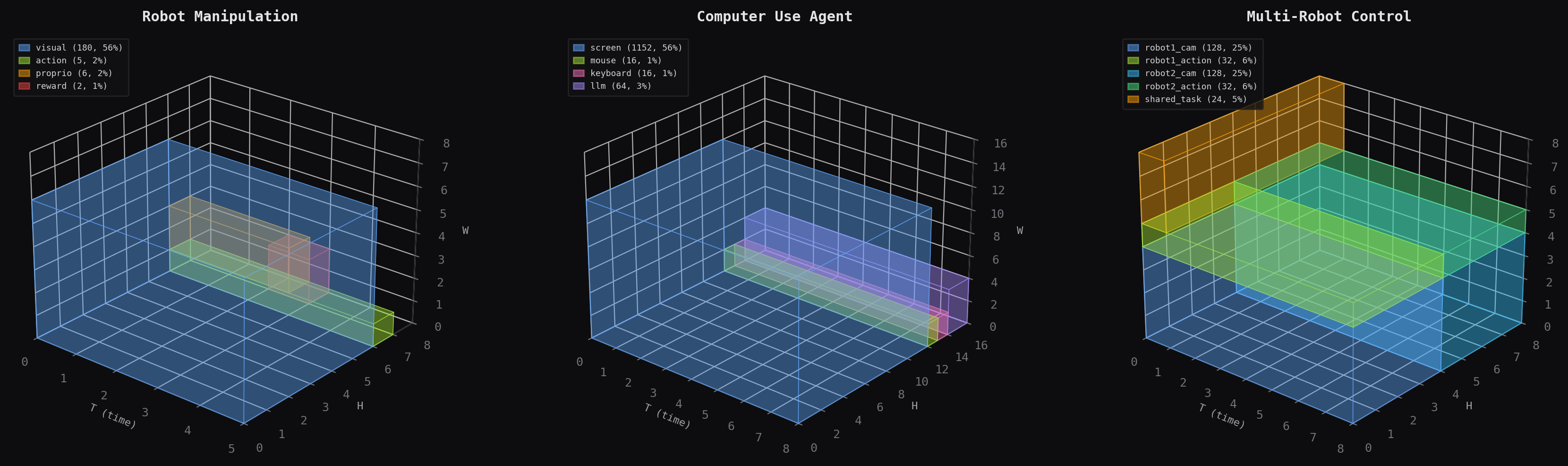
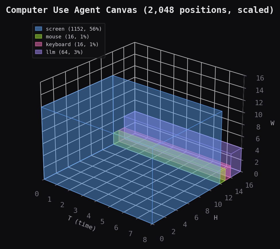
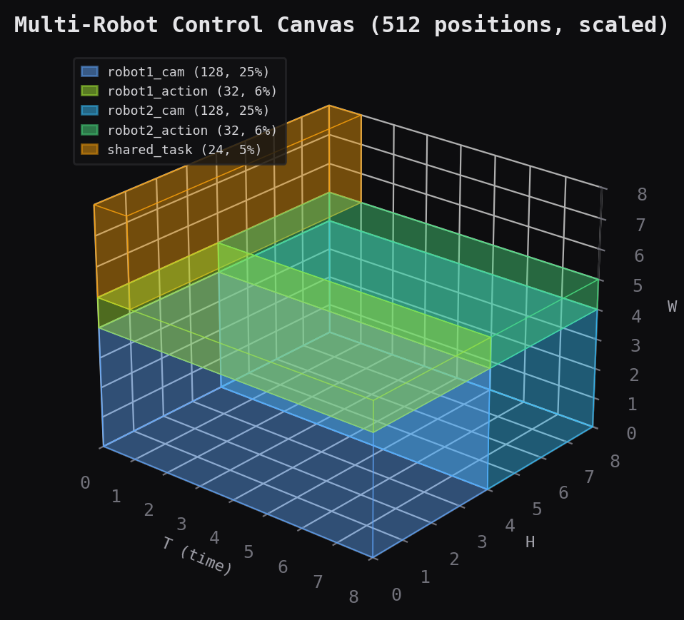
Canvas allocations for robot manipulation, computer use, and multi-robot control. Each colored block is a modality region on the 3D spatiotemporal grid.
The idea
Prompt engineering gives LLMs structured context — few-shot examples, system instructions, tool descriptions — so they produce better outputs. Canvas engineering does the same thing one level deeper: it gives diffusion models structured latent space so they learn better representations. A diffusion transformer's latent tensor is just a flat bag of positions. canvas-engineering turns it into a typed workspace by letting you declare:
- What each region means —
RegionSpecwith bounds, temporal frequency, loss weight, input/output role - How regions interact —
CanvasTopologyas a directed graph of attention operations with temporal constraints - How fast each region runs —
periodmaps canvas timesteps to real-world frames, so a "thought" region at period=4 and a "perception" region at period=1 coexist on the same canvas
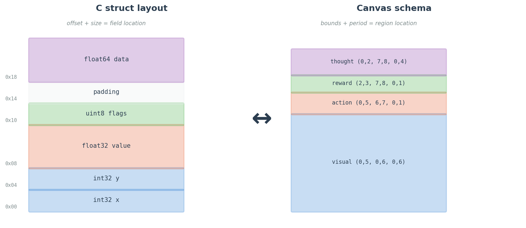
This is literally a type system. region_indices() is an offset calculation. loss_weight_mask() is type-directed codegen. The topology is a calling convention. Two agents with the same canvas schema can share latent state directly — no tokenization, no encoding — because the schema tells you what every position means.
The library has two orthogonal pieces, validated over 26 experiments and 236 training runs:
1. The canvas: structured multimodal latent space
Large video diffusion models (CogVideoX, Mochi, Wan) generate video. The spatiotemporal canvas extends them to do things — predict robot actions, estimate rewards, process proprioception — by placing heterogeneous modalities on a shared 3D grid with dedicated encoders and decoders. You design the schema, the model attends over everything.
2. Looped attention: weight-sharing regularization
Looped attention iterates transformer blocks multiple times with learned iteration embeddings. The empirical result: 1.73x parameter efficiency over matched-depth models (p<0.001) through weight-sharing regularization (fixed-point convergence, cosine similarity 0.926 → 0.996). A frozen CogVideoX-2B backbone + 350K trainable loop parameters outperforms 11.5M unfrozen parameters on action prediction. 3 loops is optimal.
What looping is not: iterative reasoning -- at least not yet. Three independent experiments falsified that hypothesis (p=0.97, p>0.05, p>0.05). The benefit is regularization, not reasoning depth, not at the limited scale I tested anyway... tho I'm skeptical.
Quick start
pip install canvas-engineering
Graft looped attention onto CogVideoX-2B
from canvas_engineering import graft_looped_blocks, CurriculumScheduler
from diffusers import CogVideoXTransformer3DModel
import torch

# Load pretrained video diffusion model
transformer = CogVideoXTransformer3DModel.from_pretrained(
    "THUDM/CogVideoX-2b", subfolder="transformer", torch_dtype=torch.bfloat16
)

# Graft 3-loop attention onto all 30 frozen DiT blocks
looped_blocks, action_head = graft_looped_blocks(
    transformer,
    max_loops=3,       # 3 is optimal (empirically validated)
    freeze="full",     # freeze backbone, train only loop params
    action_dim=7,      # 6DOF end-effector + gripper
)

# Only 350K params to optimize
optimizer = torch.optim.AdamW(
    [p for b in looped_blocks for p in b.parameters() if p.requires_grad]
    + list(action_head.parameters()),
    lr=1e-4,
)

# Curriculum: gradually ramp from 1 to 3 loops during training
scheduler = CurriculumScheduler(max_loops=3, total_steps=5000)
That's it. The frozen 1.69B-parameter backbone now loops its computation 3 times per forward pass, with learned iteration embeddings that cost 0.02% of the model.
How looped attention works
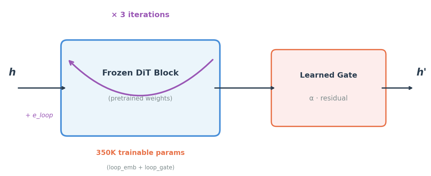
Zero-init safety: Loop embeddings start at zero. At initialization, the model behaves identically to the pretrained backbone. No distribution shift. Safe to graft onto any frozen model.
Gradient checkpointing: Multi-loop training fits in 40GB VRAM by recomputing activations on the backward pass (per-loop, not per-block).
How the canvas works
A canvas is a 3D grid (T, H, W) where different regions handle different modalities. This is the omnimodal I/O layer — it's what lets a video model also predict actions, read proprioception, and estimate reward.
from canvas_engineering import CanvasLayout, SpatiotemporalCanvas

# Robot manipulation canvas
layout = CanvasLayout(
    T=5, H=8, W=8, d_model=256,
    regions={
        "visual":  (0, 5, 0, 6, 0, 6),    # 180 positions — video patches
        "action":  (0, 5, 6, 7, 0, 1),    #   5 positions — per-frame actions
        "reward":  (2, 3, 7, 8, 0, 1),    #   1 position  — scalar reward
    },
    t_current=2,  # t >= 2 is future (diffusion output)
)

canvas = SpatiotemporalCanvas(layout)
batch = canvas.create_empty(batch_size=4)          # (4, 320, 256)
batch = canvas.place(batch, visual_embs, "visual") # write video patches
actions = canvas.extract(batch, "action")          # read action predictions
3D region allocation for a robot manipulation canvas. Each colored block is a modality occupying a subvolume of the (T, H, W) grid.
Built-in examples for robot manipulation, computer use agents, and multi-robot control:
# Computer use agent: screen pixels + mouse + keyboard + LLM steering
layout = CanvasLayout(
    T=16, H=32, W=32, d_model=768,
    regions={
        "screen":   (0, 16, 0, 24, 0, 24),     # 9,216 positions (56%)
        "mouse":    (0, 16, 24, 26, 0, 4),      #   128 positions
        "keyboard": (0, 16, 26, 28, 0, 4),      #   128 positions
        "llm":      (0, 16, 28, 32, 0, 8),      #   512 positions
    },
)
# → 16,384 total positions, bandwidth-proportional allocation
Why 3 loops?
From a 12-condition grid ablation on CogVideoX-2B with real Bridge V2 robot video (36 runs, $152 compute):
Action Loss (lower = better)
                Frozen         Half-frozen     Unfrozen
                (350K params)  (3.7M params)   (11.7M params)
  1 loop        0.121          0.115           0.108
  2 loops       0.140          0.119           0.112
  3 loops       0.073 ◀ BEST   0.107           0.088
  4 loops       0.104          0.137           0.124
3 loops wins at every freeze level. The frozen 3-loop condition (350K params) beats every unfrozen condition (11.5M+ params). 4 loops consistently regresses from 3.
Freeze level doesn't affect action loss at all (marginals: 0.109 vs 0.108, p=0.72). It only affects video generation quality (8-9x gap on diffusion loss).
Declarative region frequency
Canvas regions can operate at different real-world frequencies. A RegionSpec declares per-region semantics — temporal frequency, loss participation, and loss weight — as first-class properties.
from canvas_engineering import CanvasLayout, RegionSpec

layout = CanvasLayout(
    T=16, H=32, W=32, d_model=768,
    regions={
        "screen": (0, 16, 0, 24, 0, 24),         # raw tuple — period=1 default

        "mouse": RegionSpec(
            bounds=(0, 16, 24, 26, 0, 4),
            period=1, loss_weight=2.0,             # high-freq, emphasize accuracy
        ),
        "thought": RegionSpec(
            bounds=(0, 4, 28, 32, 0, 8),
            period=4, loss_weight=1.0,             # low-freq: 4 slots → frames 0,4,8,12
        ),
        "task_prompt": RegionSpec(
            bounds=(0, 1, 26, 28, 0, 4),
            is_output=False,                       # input-only conditioning, no loss
        ),
    },
)

# Per-position loss weighting — respects is_output and loss_weight
weights = layout.loss_weight_mask("cuda")          # (N,) tensor
loss = (per_position_loss * weights).sum() / weights.sum()

# Frame mapping between canvas time and real-world time
layout.real_frame("thought", canvas_t=2)           # → 8
layout.canvas_frame("thought", real_t=8)           # → 2
layout.canvas_frame("thought", real_t=7)           # → None (not aligned)
Raw tuples auto-wrap as RegionSpec(bounds=tuple) with defaults — full backward compatibility. All existing code continues to work unchanged.
RegionSpec fields:
| Field | Default | Meaning |
|---|---|---|
bounds |
(required) | (t0, t1, h0, h1, w0, w1) spatial-temporal extent |
period |
1 |
Canvas frames per real-world update (1 = every frame) |
is_output |
True |
Whether this region participates in diffusion loss |
loss_weight |
1.0 |
Relative loss weight for positions in this region |
Non-Euclidean connectivity
Canvas regions don't have to interact via Euclidean adjacency. A CanvasTopology declaratively specifies which block-to-block attention operations are performed per step. Each Connection is a discrete cross-attention op: src tokens query against dst keys/values.
from canvas_engineering import Connection, CanvasTopology

# Declarative: define the full attention compute DAG as data
topology = CanvasTopology(connections=[
    # Self-attention within each region
    Connection(src="robot1_cam",    dst="robot1_cam"),
    Connection(src="robot1_action", dst="robot1_action"),
    Connection(src="robot2_cam",    dst="robot2_cam"),
    Connection(src="robot2_action", dst="robot2_action"),
    Connection(src="shared_task",   dst="shared_task"),

    # Causal: each robot's camera informs its own actions
    Connection(src="robot1_action", dst="robot1_cam"),
    Connection(src="robot2_action", dst="robot2_cam"),

    # Coordination: robots see each other's cameras
    Connection(src="robot1_cam", dst="robot2_cam", weight=0.5),
    Connection(src="robot2_cam", dst="robot1_cam", weight=0.5),

    # Hub: shared task reads from cameras, actions read from task
    Connection(src="shared_task",   dst="robot1_cam"),
    Connection(src="shared_task",   dst="robot2_cam"),
    Connection(src="robot1_action", dst="shared_task"),
    Connection(src="robot2_action", dst="shared_task"),
])

# Generate attention mask or iterate over ops
mask = topology.to_attention_mask(layout)  # (N, N) float
ops = topology.attention_ops()             # [(src, dst, weight), ...]
Convenience constructors for common patterns:
CanvasTopology.dense(["a", "b", "c"])          # fully connected (standard transformer)
CanvasTopology.isolated(["a", "b", "c"])       # block-diagonal (no cross-region)
CanvasTopology.hub_spoke("task", ["r1", "r2"]) # star topology
CanvasTopology.causal_chain(["obs", "plan", "act"])  # A → B → C
CanvasTopology.causal_temporal(["obs", "act"]) # same-frame self + prev-frame cross
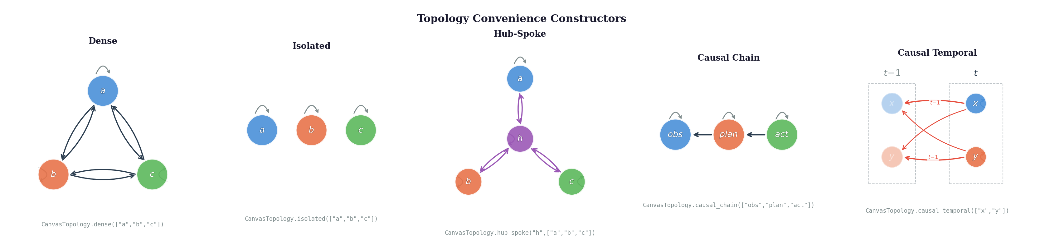
The topology is the compute graph of attention operations — not a soft mask on dense attention. Block self-attention is one special case. Dense is another. The interesting cases are structured DAGs that mirror the causal/information-flow structure of your problem.
Temporal connectivity
Connections can constrain which timesteps participate in each attention op. By default, all timesteps see all timesteps (dense in time). With temporal offsets, you get causal chains over time, same-frame-only constraints, or sliding windows.
# Default: all timesteps (backward compatible)
Connection(src="cam", dst="action")

# Same-frame only: no temporal leakage
Connection(src="cam", dst="action", t_src=0, t_dst=0)

# Previous frame cross-attention: action at t queries obs at t-1
Connection(src="action", dst="obs", t_src=0, t_dst=-1)

# Full temporal self-attention (explicit)
Connection(src="thought", dst="thought", t_src=None, t_dst=None)
Semantics: t_src and t_dst are relative offsets from a shared reference frame. The mask generator iterates over all reference frames and pairs positions at ref + t_src with positions at ref + t_dst. Out-of-bounds timesteps are silently skipped.
t_src |
t_dst |
Behavior |
|---|---|---|
None |
None |
All src ↔ all dst (dense in time) |
0 |
0 |
Same-frame only |
0 |
-1 |
Src at current frame queries dst at previous frame |
None |
0 |
All src timesteps query dst at each reference frame |
The causal_temporal constructor gives you same-frame self-attention + previous-frame cross-attention for all regions — no future leakage, but full temporal context.
Attention function types
Not all connections should use the same attention mechanism. A Connection can declare its fn — the type of function used for that edge. Regions can also set default_attn — a default for all outgoing connections. The schema declares intent; execution is backend-dependent.
from canvas_engineering import CanvasLayout, RegionSpec, Connection, CanvasTopology

layout = CanvasLayout(
    T=8, H=16, W=16, d_model=512,
    regions={
        # Region defaults: what kind of attention makes sense for this modality?
        "visual":  RegionSpec(bounds=(0,8, 0,12, 0,12), default_attn="cross_attention"),
        "proprio": RegionSpec(bounds=(0,8, 12,13, 0,2), default_attn="linear_attention"),
        "thought": RegionSpec(bounds=(0,4, 13,15, 0,4), default_attn="mamba"),
        "goal":    RegionSpec(bounds=(0,1, 15,16, 0,4), default_attn="cross_attention",
                              is_output=False),
    },
)

topology = CanvasTopology(connections=[
    # Self-attention (uses each region's default_attn)
    Connection(src="visual",  dst="visual"),           # → cross_attention
    Connection(src="proprio", dst="proprio"),           # → linear_attention
    Connection(src="thought", dst="thought"),           # → mamba
    Connection(src="goal",    dst="goal"),              # → cross_attention

    # Cross-region with explicit fn overrides
    Connection(src="visual",  dst="goal", fn="gated"),       # optional conditioning
    Connection(src="thought", dst="visual", fn="perceiver"), # compress 864 visual tokens
    Connection(src="proprio", dst="visual", fn="pooling"),   # just need a summary
    Connection(src="thought", dst="thought", fn="copy",      # direct latent relay
               t_src=0, t_dst=-1),                           # from previous frame
])

# Resolve: returns (src, dst, weight, fn) with defaults applied
ops = topology.attention_ops(layout)
# [("visual", "visual", 1.0, "cross_attention"),
#  ("proprio", "proprio", 1.0, "linear_attention"),
#  ("thought", "thought", 1.0, "mamba"),
#  ...]
Resolution order: connection.fn (if set) → region.default_attn (if layout provided) → "cross_attention" (global default). Fully backward compatible — existing code without fn or default_attn resolves to standard cross-attention.
The lineup
Every connection function type represents a different theory of how information should flow between regions. The schema declares intent; the executor decides implementation.
| Type | Family | Complexity | Best for |
|---|---|---|---|
cross_attention |
Dot-product | O(NM) | General-purpose, content-based selection |
linear_attention |
Dot-product | O(N+M) | Low-dimensional or high-frequency streams |
cosine_attention |
Dot-product | O(NM) | Stable gradients, no temperature scaling |
sigmoid_attention |
Dot-product | O(NM) | Non-exclusive / multi-label attention |
gated |
Gating | O(NM) | Optional conditioning (goals, instructions) |
perceiver |
Compression | O(NK) | Large dst regions compressed through bottleneck |
pooling |
Compression | O(N+M) | Scalar/low-dim conditioning signals |
copy |
Transfer | O(N) | Direct latent sharing, broadcast regions |
mamba |
State-space | O(N) | Long temporal sequences, causal connections |
rwkv |
State-space | O(N) | Temporal connections with learned decay |
hyena |
Convolution | O(N log N) | Sub-quadratic long-range via FFT |
sparse_attention |
Sparse | O(NK) | Selective binding to specific positions |
local_attention |
Sparse | O(NW) | Spatially local interactions (neighboring patches) |
none |
Meta | O(0) | Ablation — edge declared but disabled |
random_fixed |
Meta | O(NK) | Baseline — does learned structure matter? |
mixture |
Meta | O(NK) | MoE-style routing for multi-modal hubs |
Design recipes
Robot manipulation — vision-heavy, low-latency actions:
"visual":  default_attn="cross_attention"    # full attention for spatial reasoning
"proprio": default_attn="linear_attention"   # 12D joint state, no need for O(N²)
"action":  default_attn="cross_attention"    # content-based selection from visual
# visual → action: cross_attention (which visual patches matter for this action?)
# proprio → action: pooling (just need the joint state vector)
Embodied agent with memory — long-horizon, selective recall:
"perception": default_attn="cross_attention"
"memory":     default_attn="mamba"            # O(N) sequential over long history
"policy":     default_attn="cross_attention"
# memory → perception: gated (decide whether to incorporate memory at all)
# perception → memory: perceiver (compress percepts into fixed-size memory)
Multi-agent coordination — shared latent space:
"agent_a.thought": default_attn="rwkv"       # causal temporal within agent
"agent_b.thought": default_attn="rwkv"
"shared_task":     default_attn="cross_attention"
# agent_a.thought → shared_task: cross_attention (selective broadcast)
# shared_task → agent_b.thought: gated (selective incorporation)
# agent_a.thought → agent_b.thought: copy (direct latent relay)
Vision transformer backbone — drop-in structured attention:
"cls_token":  default_attn="cross_attention"
"patches":    default_attn="local_attention"   # each patch attends locally
"readout":    default_attn="cross_attention"
# cls_token → patches: cross_attention (global aggregation)
# patches → patches: local_attention (spatial locality)
# readout → cls_token: pooling (single vector summary)
Semantic types and transfer distance
Each canvas region represents a modality — RGB video, joint angles, reward, language. RegionSpec lets you declare the modality's semantic type as a human-readable string and a frozen embedding vector from a fixed model. This turns modality compatibility from a human judgment call into a computable quantity.
from canvas_engineering import RegionSpec, transfer_distance

cam = RegionSpec(
    bounds=(0, 8, 0, 12, 0, 12),
    semantic_type="RGB video 224x224 30fps from front-facing monocular camera",
    semantic_embedding=embed("RGB video 224x224 30fps from front-facing monocular camera"),
    embedding_model="openai/text-embedding-3-small",  # fixed, declared
)

depth = RegionSpec(
    bounds=(0, 8, 0, 12, 0, 12),
    semantic_type="Metric depth map 224x224 from front-facing monocular camera",
    semantic_embedding=embed("Metric depth map 224x224 from front-facing monocular camera"),
)

joints = RegionSpec(
    bounds=(0, 8, 12, 13, 0, 1),
    semantic_type="7-DOF joint angles at 30Hz",
    semantic_embedding=embed("7-DOF joint angles at 30Hz"),
)

transfer_distance(cam, depth)    # ~0.15 — cheap to bridge (1-2 layers)
transfer_distance(cam, joints)   # ~0.65 — expensive (full MLP adapter)
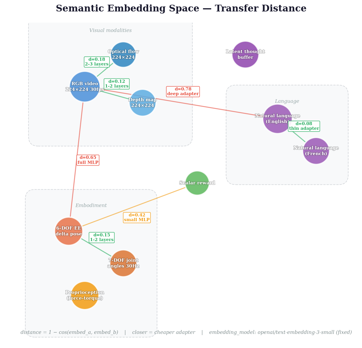
Why this matters: If canvas schemas produce stable latent representations (an empirical hypothesis we're testing), then semantic embedding distance approximates the real cost of bridging two modalities — how many adapter layers, how much data. The embedding model must be fixed and declared so distances are comparable across time and projects.
Canvas schemas
A CanvasSchema bundles layout + topology into a single portable, serializable object — the complete type signature for a canvas-based model.
from canvas_engineering import CanvasSchema, CanvasLayout, RegionSpec, CanvasTopology, Connection

schema = CanvasSchema(
    layout=CanvasLayout(
        T=8, H=16, W=16, d_model=256,
        regions={
            "visual": RegionSpec(
                bounds=(0, 8, 0, 12, 0, 12),
                semantic_type="RGB video 224x224",
                semantic_embedding=(0.12, -0.05, ...),
            ),
            "action": RegionSpec(
                bounds=(0, 8, 12, 14, 0, 2),
                loss_weight=2.0,
                semantic_type="6-DOF end-effector + gripper",
                semantic_embedding=(0.31, 0.08, ...),
            ),
        },
    ),
    topology=CanvasTopology(connections=[
        Connection(src="visual", dst="visual"),
        Connection(src="action", dst="visual"),
        Connection(src="action", dst="action"),
    ]),
    metadata={"model": "CogVideoX-2B", "data": "bridge_v2"},
)

# Serialize — the schema is the complete declaration
schema.to_json("robot_v1.json")
loaded = CanvasSchema.from_json("robot_v1.json")

# Find compatible regions across two schemas
pairs = schema.compatible_regions(other_schema, threshold=0.3)
# → [("visual", "camera", 0.04), ("action", "gripper_cmd", 0.12)]
The schema file is human-readable JSON. It declares everything needed to interpret a canvas tensor: geometry, region semantics, connectivity, and modality types. Two models with the same schema can share latent state directly.
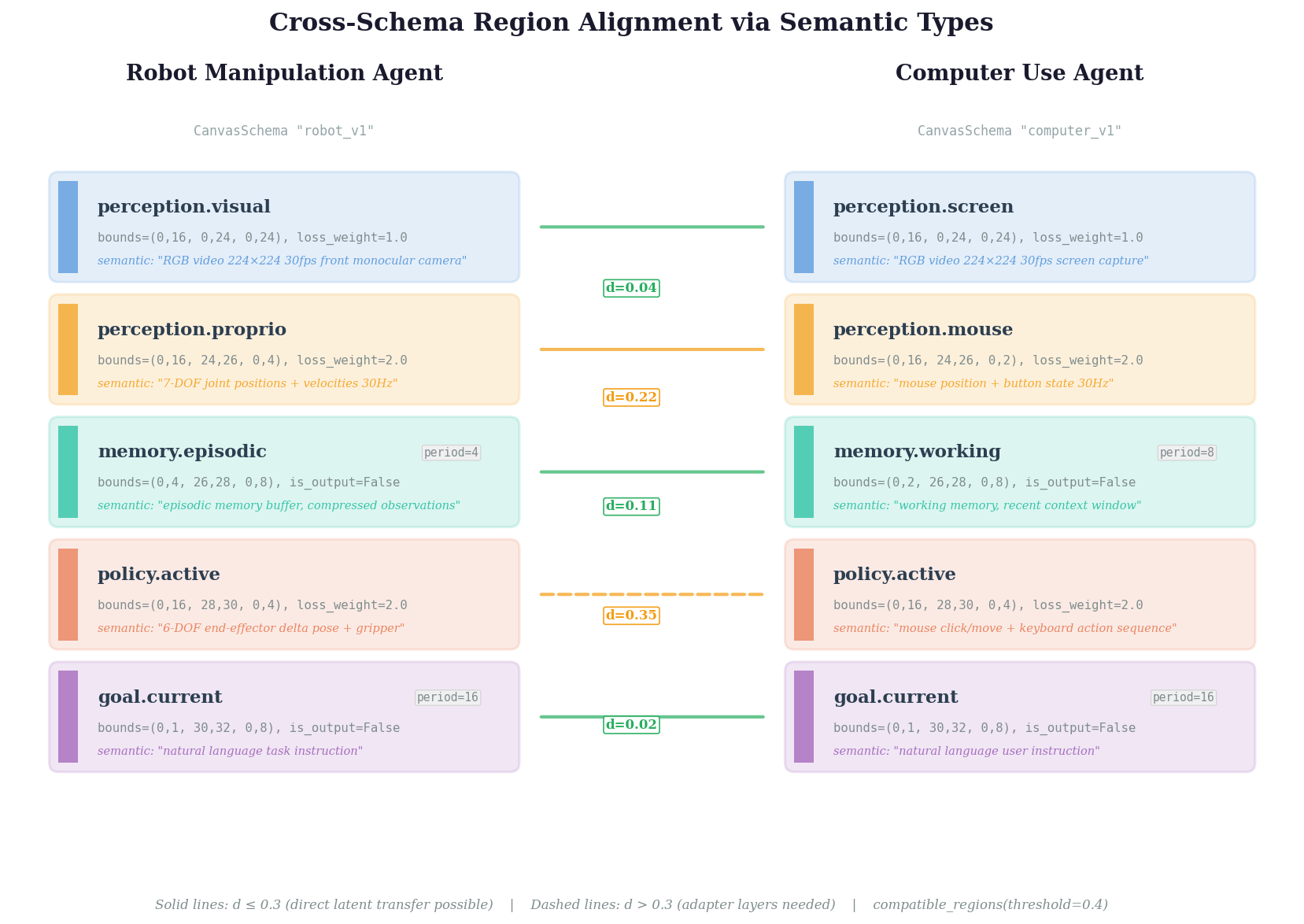
Two agents with different canvas schemas. compatible_regions() finds semantically aligned region pairs — solid lines indicate direct latent transfer is possible, dashed lines require adapter layers.
API reference
| Module | What it does |
|---|---|
| Canvas (omnimodal I/O) | |
CanvasLayout |
Declarative 3D canvas geometry with named regions |
RegionSpec |
Per-region semantics: frequency, loss weight, output participation |
SpatiotemporalCanvas |
Canvas tensor ops: create_empty, place, extract |
Connection |
Single attention op with temporal offsets and function type (fn) |
CanvasTopology |
Declarative DAG of attention ops with resolve_fn() dispatch |
ATTENTION_TYPES |
Registry of 16 declared attention function types |
transfer_distance() |
Cosine distance between semantic type embeddings |
CanvasSchema |
Portable bundle: layout + topology + metadata, JSON-serializable |
ActionHead |
MLP decoder: latent channels → robot actions |
| Looped attention (adaptive compute) | |
LoopedBlockWrapper |
Wrap any transformer block for looped execution |
graft_looped_blocks() |
One-line grafting onto CogVideoX (auto-detects block type) |
freeze_full() / freeze_half() |
Freeze strategies for the backbone |
CurriculumScheduler |
Ramp loop count 1→3 during training |
SharpeningSchedule |
Progressive attention sharpening across loops (soft→sharp) |
| Utilities | |
save_loop_checkpoint() |
Save only loop params (~0.1% of model, ~1.4 MB) |
Freeze strategies
| Strategy | What's frozen | Trainable | Action loss | Diffusion loss | Use when |
|---|---|---|---|---|---|
"full" |
Everything except loops | 350K | 0.073 | 1.48 | Max efficiency, action-only tasks |
"half" |
Only patch_embed |
3.7M | 0.107 | 0.19 | Good video + good actions |
"none" |
Nothing | 11.7M | 0.088 | 0.18 | Full fine-tuning, compute available |
Progressive sharpening
Loop-indexed inverse temperature for bridging the soft→sharp attention discontinuity:
from canvas_engineering import SharpeningSchedule

schedule = SharpeningSchedule(max_loops=3, beta_min=1.0, beta_max=4.0)

# Loop 0: beta=1.0 (soft, broad gradients)
# Loop 1: beta=2.5 (medium)
# Loop 2: beta=4.0 (sharp, precise attention)
Early loops train Q/K matrices via gradient flow. Later loops exploit trained structure with near-discrete attention. Empirically: mild sharpening (beta→2) gives 1.30x F1 on contact detection; aggressive (beta→8) hurts.
What looping is NOT
We tested three cortical-computation hypotheses rigorously. Two are falsified:
| Hypothesis | Result | Evidence |
|---|---|---|
| Looping enables iterative reasoning | Falsified | 3 independent nulls (p=0.97, p>0.05, p>0.05) |
| Shared canvas creates multi-modal binding | Falsified | Joint prediction 19% worse (p<0.0001) |
| Token allocation follows power laws | Borderline | R^2=0.902 but alpha=0.011 (doubling tokens = 0.8%) |
The looping benefit is weight-sharing regularization (parameter efficiency, fixed-point convergence, lower variance), not iterative reasoning. The omnimodal capability comes from the canvas architecture (multi-encoder/multi-decoder), not from the looping.
Compositional types and hierarchical coarse-graining
compile_schema accepts nested dataclasses, not just flat field lists. Every nested type automatically gets a coarse-grained field — a compressed representation at the child's path that bottlenecks cross-level attention. This means a parent with 1000 children doesn't create O(N²) cross-entity connections — interactions route through compact coarse-grained fields.
from dataclasses import dataclass, field as dc_field
from canvas_engineering import Field, compile_schema

@dataclass
class Sensor:
    __coarse__ = Field(2, 4)          # when viewed from parent: 2×4 region
    rgb: Field = Field(12, 12)
    depth: Field = Field(6, 6)
    lidar: Field = Field(4, 8)

@dataclass
class Arm:
    joints: Field = Field(1, 7)
    force_torque: Field = Field(1, 6)
    gripper: Field = Field(1, 2, loss_weight=2.0)

@dataclass
class SurgicalRobot:
    # Per-child coarse-grained size via metadata
    sensor: Sensor = dc_field(default_factory=Sensor)
    left_arm: Arm = dc_field(
        default_factory=Arm,
        metadata={"coarse": Field(2, 4)},  # override for this edge
    )
    right_arm: Arm = dc_field(default_factory=Arm)
    safety: Field = Field(2, 4, loss_weight=5.0)

bound = compile_schema(SurgicalRobot(), d_model=256)
The compiled schema has:
sensor(2×4 coarse-grained field) ↔sensor.rgb,sensor.depth,sensor.lidarleft_arm(2×4 override) ↔left_arm.joints,left_arm.force_torque,left_arm.gripperright_arm(1×1 default) ↔ its child fieldssafetyconnects to all coarse-grained fields (via parent-level intra connections)
Cross-level attention: safety ↔ sensor (coarse) ↔ sensor.rgb. The arms don't see each other's internal joint states — only through the parent's safety field and their own coarse-grained representations.
Arrays: fleets, teams, portfolios
Arrays of entities each get their own coarse-grained field. The parent sees only the compact representations:
@dataclass
class Vehicle:
    __coarse__ = Field(4, 4)          # each vehicle → 4×4 summary
    camera: Field = Field(8, 8)
    lidar: Field = Field(4, 8)
    plan: Field = Field(2, 4)
    action: Field = Field(1, 4, loss_weight=2.0)

@dataclass
class Fleet:
    dispatch: Field = Field(4, 4)
    vehicles: list = dc_field(default_factory=list)

fleet = Fleet(vehicles=[Vehicle() for _ in range(50)])
bound = compile_schema(fleet, d_model=256)
# 50 vehicles × (4×4 coarse + 4 internal fields) = manageable
# dispatch ↔ vehicles[i] (coarse) ↔ vehicles[i].camera, etc.
# vehicles[0] does NOT directly attend to vehicles[1].camera
Without coarse-graining, 50 vehicles with dense cross-attention is 50² × fields² connections. With coarse-graining, each vehicle interacts through its 4×4 summary — O(50 × 16) instead of O(50² × 100+).
Hierarchical composition for world models
Deep nesting creates a chain of coarse-grained fields at each level:
@dataclass
class MacroEconomy:
    __coarse__ = Field(2, 4)
    gdp: Field = Field(1, 2)
    inflation: Field = Field(1, 2)
    employment: Field = Field(1, 4)
    # ... 50+ fields

@dataclass
class Country:
    __coarse__ = Field(4, 4)
    macro: MacroEconomy = dc_field(default_factory=MacroEconomy)
    politics: Field = Field(2, 8)      # or another nested type
    demographics: Field = Field(1, 4)

@dataclass
class World:
    us: Country = dc_field(default_factory=Country)
    cn: Country = dc_field(default_factory=Country)
    regime: Field = Field(4, 4)

bound = compile_schema(World(), d_model=64)
# regime ↔ us (4×4 coarse) ↔ us.macro (2×4 coarse) ↔ us.macro.gdp
# us (coarse) ↔ cn (coarse) — countries see each other's summaries
# us.macro.gdp does NOT directly attend to cn.macro.inflation
The attention path from US GDP to Chinese inflation goes: us.macro.gdp → us.macro (coarse) → us (coarse) → regime ↔ cn (coarse) → cn.macro (coarse) → cn.macro.inflation. Each level compresses, so the model learns hierarchical abstractions — not because we told it to, but because the topology forces it.
Examples
examples/
├── quickstart.py           # 30-line graft-and-train
├── graft_cogvideox.py      # Full CogVideoX grafting with training loop
├── define_canvas.py        # Canvas layouts for 3 applications
└── train_bridge_v2.py      # Real robot data training
Installation
# Core (canvas + looped blocks)
pip install canvas-engineering

# With CogVideoX support
pip install canvas-engineering[cogvideox]

# With video dataset loading
pip install canvas-engineering[data]

# Development
pip install canvas-engineering[dev]
Requires Python 3.9+ and PyTorch 2.0+.
Paper
Looped Attention in Video Diffusion Transformers: 26 Experiments on What Works, What Doesn't, and Why
Jacob Valdez and Claude Opus 4.6
Paper PDF | Video | Full experiment data
License
Apache 2.0
Release history Release notifications | RSS feed


Download files
Download the file for your platform. If you're not sure which to choose, learn more about installing packages.
Source Distribution
Built Distribution
Filter files by name, interpreter, ABI, and platform.
If you're not sure about the file name format, learn more about wheel file names.
Copy a direct link to the current filters
File details
Details for the file canvas_engineering-0.1.4.tar.gz.
File metadata
- Download URL: canvas_engineering-0.1.4.tar.gz
- Upload date:
- Size: 89.5 kB
- Tags: Source
- Uploaded using Trusted Publishing? No
- Uploaded via: twine/6.2.0 CPython/3.12.12
File hashes
| Algorithm | Hash digest | |
|---|---|---|
| SHA256 |
a6a84a7a541c9341236e9d18ba84615dfe3fb188b33f0327cb14e749cc849309
|
|
| MD5 |
64823e9595a80f51aad4a272c6d81ca7
|
|
| BLAKE2b-256 |
2b8d42fee864ab8825b32af1cd6ec6350bab006847fcd66b1c58ce52df4886c9
|
File details
Details for the file canvas_engineering-0.1.4-py3-none-any.whl.
File metadata
- Download URL: canvas_engineering-0.1.4-py3-none-any.whl
- Upload date:
- Size: 56.7 kB
- Tags: Python 3
- Uploaded using Trusted Publishing? No
- Uploaded via: twine/6.2.0 CPython/3.12.12
File hashes
| Algorithm | Hash digest | |
|---|---|---|
| SHA256 |
51426b3d13ae94fa25c12c5a81b623b53775d463fd1f76a527f4c430babe99d4
|
|
| MD5 |
e419de77379003b7101d5ff87cc09a5d
|
|
| BLAKE2b-256 |
53114312a1a5c95080155298fb7bad48a8066d722c33f164429fd061b8e34f09
|


