Python program for finding catenary shapes and mass densities

Project description
catenary-solver v1.0.0
Python program for finding catenary shapes and mass densities
This program was created as a part of the Summer Undergraduate Reasearch Experience at Carthage College. The goal of the project was to answer the question "Is it possible to find the mass density of a hanging cable given its shape?", which is the inverse of the normal "forward" problem that asks if it is possible to find the shape of a hanging cable given its mass density. The program contains functions that compute the answers to both the forward problem and the inverse problem.
The full source code is provided with annotations on how to use each function, and what is happening as the program runs. For convenience, here are the main functions within the program and how to use them.
These functions find the shape a cable would make if hung from its ends given horizontal distance between the ends, the vertical distance between the ends, the length of the cable, and the mass density of the cable with respect to arc length. There are two more parameters that are brute-forced to create the desired curve. These are the initial slope of the curve, as well as the horizonal tension in the curve.
For the Forward Problem
find_parameters()
-- Main function to brute force h (horizontal tension / 9.8) and the initial slope of a desired cable, given characteristics of the curve
| required/optional | parameter, type | description |
|---|---|---|
| required | dens, function: | user-created function dens() that takes one argument and returns the mass density of the user's cable at specified arc length (if using free-hanging model) or horizontal distance (if using loaded model) |
| required | xdist, float: | desired horizontal distance between the two endpoints of the cable |
| required | ydist, float: | desired vertical distance between the two endpoints of the cable |
| required | length, float: | desired length of cable |
| optional, default=None | guess_h, float: | allows the user to set a starting value when searching for h, may decrease search times |
| optional, default=None | guess_dydx, float: | allows the user to set a starting value when searching for the initial slope of the curve, not recommended |
| optional, default=.01 | thresh, float: | represents the maximum x/y-distance a generated curve's endpoint can be compared to the desired endpoint in order for the program to count a curve as successful, lower values take longer/more loops but give generally more accurate results |
| optional, default=500 | max_attempts, int: | the maximum number of loops/curves to generate in an attempt to find the desired curve |
| optional, default=False | debug, boolean: | if set to True, prints information about each curve generated while searching for the correct curve |
| optional, default=hanging | type, function: | specifies if the free-hanging or loaded cable function should be used to solve the differential equation |
find_catenary(dens, xdist, ydist, length, thresh=.01, max_attempts=500, debug=False)
-- Essentially calls find_parameters() with specific arguments to make compute time faster using scaling. Used to find the shape of a free-hanging cable.
| required/optional | parameter, type | description |
|---|---|---|
| required | dens, function: | user-created function dens() that takes one argument and returns the mass density of the user's cable at specified arc length (if using free-hanging model) or horizontal distance (if using loaded model) |
| required | xdist, float: | desired horizontal distance between the two endpoints of the cable |
| required | ydist, float: | desired vertical distance between the two endpoints of the cable |
| required | length, float: | desired length of cable |
| optional, default=.01 | thresh, float: | represents the maximum x/y-distance a generated curve's endpoint can be compared to the desired endpoint in order for |
| the program to count a curve as successful, lower values take longer/more loops but give generally more accurate results | ||
| optional, default=500 | max_attempts, int: | the maximum number of loops/curves to generate in an attempt to find the desired curve |
| optional, default=False | debug, boolean: | if set to True, prints information about each curve generated while searching for the correct curve |
find_loaded_catenary(dens, xdist, ydist, length, thresh=.01, max_attempts=500, debug=False)
-- the exact same as find_catenary(), but uses type=loaded in the find_parameters() function call to solve the loaded cable diff eq (e.g. for a cable supporting a road directly beneath it)
CatSolution Object
All three of these functions return a CatSolution object, which has the following members:
| member | description |
|---|---|
| status, int: | -1 = failed, desired cable length is not long enough to reach desired cable endpoint |
| 0 = success, curve was found with endpoint within desired threshold | |
| 1 = maximum number of loops occurred or variable increments are too small, returns the curve with the closest distance from desired endpoint to simulated endpoint | |
| message, string: | describes result of attempt to find curve |
| type, string: | "Free-hanging" or "Loaded", depending on whether find_catenary() or find_loaded_catenary() was called |
| h, float: | h found as a result of attempt to find curve |
| idydx, float: | initial slope found as a result of attempt to find curve |
| x, array of floats: | list of x-coordinates that make up curve |
| y, array of floats: | list of y-coordinates that make up curve |
It is recommended to use find_catenary() or find_loaded_catenary() and not find_parameters(). To create the density function, define a function that inputs an arc length and outputs the density at that arc length. For example, for a catenary of constant mass density, one might define:
def density1(s):
  return 2
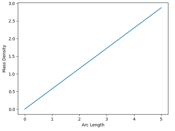
For a catenary with a linearly increasing mass density:
def density2(s):
  return s
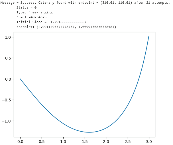
The resulting shape could then be obtained and plotted through
from catsolver.forward import find_catenary

cat = find_catenary(density2, 3, 1, 5)
You can print the CatSolution object to output relevant information about the curve as well as plot what the resulting curve looks like with any plotting package. For example,
import matplotlib.pyplot as plt

print(cat)
plt.plot(cat.x, cat.y)
For the Inverse Problem
The following functions are designed to take in the shape of a catenary curve and output an 2D array representing arc length vs density for that shape if it was hung from its ends.
dens_from_spline()
-- outputs arc length vs density when given a spline that starts at x=0 and ends at x=xdist, output is of the form = [arc length array, density array]
| parameter, type | description |
|---|---|
| spline: | any spline-related object from scipy.interpolate(), models the curve that we want to know the mass density of |
| xdist, float: | the last x-value of the spline/curve, used to define the range to create (x, y) points from the spline |
dens_from_spline() is situational in that you need to have a spline representation of the curve on hand. However, it is also the most useful because it can process shapes that do not easily fit common functions such as x^2 or sin(x). The ideal use for this function would be to take in a spline that was generated using points on a real-life image of a catenary shape. While slightly redundant, here is an example using the curve that was generated in the previous section.
import scipy.interpolate as spi
from catsolver.inverse import dens_from_spline

splcat = spi.InterpolatedUnivariateSpline(cat.x, cat.y)
s, d = dens_from_spline(splcat, cat.x[-1])
plt.plot(s, d)
plt.xlabel('Arc Length')
plt.ylabel('Mass Density')
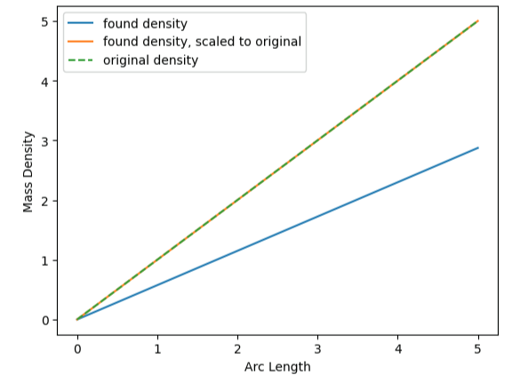
You will probably notice that the density that was found does not perfectly match the density we defined earlier (with a density equal to arc length, you would imagine the graph to be a straight line from (0, 0) to (5, 5). This is due to an underlying property of catenaries in which the shape that is created is the same for all scalar multiples of a certain density function. In other words, a cable with a density of 5 * s will make the same shape as a cable with a density of 1 * s, assuming length, x distance, and y distance stay the same. The found arc length vs density follows this rule, which can be proved through this code:
# c = scalar multiple of user-defined density, e.g. found density from dens_from_spline() = c * density used to generate curve
c = density2(5)/d[-1]
# two plots below should overlap as long as density does not start at 0
plt.plot(s, [c*d[i] for i in range(len(s))], label='found density, scaled to original')
plt.plot(s, [density2(s[i]) for i in range(len(s))], linestyle='dashed', label='original density')
dens_from_eq()
-- outputs arc length vs density when an exact function for the shape of the curve is known, also prints the equation of the x-coordinate vs density curve (NOT arc length vs density)
| parameter, type | description |
|---|---|
| x, sympy.Symbol: | x-variable in the equation of the curve |
| shape: | expression that defines the shape of the curve, e.g. shape = (x-1)**2 |
| xdist: | the last x-value to be evaluated on the shape/curve, used to define the range to create (x, y) points on the shape |
dens_from_eq() is useful if you know the shape that you want the hanging cable to make follows an easily defined function. Note that the function should start at x = 0, so you may need to shift the function using function transformations. The program will also output a warning message if the shape is not possible in the real world due to requiring negative density, but will still give a theoretical output. This is because the second derivative of the shape is negative at some point on the curve over the area being evaluated.
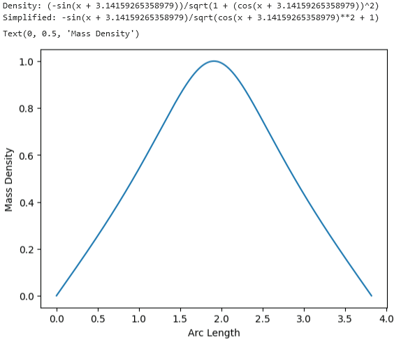
As an example, let's model the density that a cable would need to have in order to form the shape of a sin curve. In particular, we want the portion of sin(x) from pi to 2 * pi because this section is possible in the real world.
import sympy as sym
from catsolver.inverse import dens_from_eq

x = sym.Symbol('x')
s, d = dens_from_eq(x, sym.sin(x+math.pi), math.pi)
plt.plot(s, d)
plt.xlabel('Arc Length')
plt.ylabel('Mass Density')
Thats all for now! More functionality may be added in the future.
Release history Release notifications | RSS feed


Download files
Download the file for your platform. If you're not sure which to choose, learn more about installing packages.
Source Distribution
Built Distribution
Filter files by name, interpreter, ABI, and platform.
If you're not sure about the file name format, learn more about wheel file names.
Copy a direct link to the current filters
File details
Details for the file catenary_solver-1.0.0.tar.gz.
File metadata
- Download URL: catenary_solver-1.0.0.tar.gz
- Upload date:
- Size: 13.9 kB
- Tags: Source
- Uploaded using Trusted Publishing? No
- Uploaded via: twine/5.1.1 CPython/3.12.4
File hashes
| Algorithm | Hash digest | |
|---|---|---|
| SHA256 |
46fbe96404bb7d34fe8110c983cb3281c2b40e0243a6800e98932076c6fca9b4
|
|
| MD5 |
3bdf8922ebd1fea68655f45b88eb4d81
|
|
| BLAKE2b-256 |
7e4e43f4656f91f0dadbcc1c17923d0bc6a7e57023f5a2b9d769e282c32805d6
|
File details
Details for the file catenary_solver-1.0.0-py3-none-any.whl.
File metadata
- Download URL: catenary_solver-1.0.0-py3-none-any.whl
- Upload date:
- Size: 14.3 kB
- Tags: Python 3
- Uploaded using Trusted Publishing? No
- Uploaded via: twine/5.1.1 CPython/3.12.4
File hashes
| Algorithm | Hash digest | |
|---|---|---|
| SHA256 |
69a95b24d1e776fc54f888791fb225aef453c95488974fcad681d0ebc42d22a8
|
|
| MD5 |
ae0d9e7f01d5e2a0278b0e42974e4d17
|
|
| BLAKE2b-256 |
e0f16c30640de7d609a591ffef951feaf55ed0bb6c4018250a7aaf4f5481dea5
|


