Control Barrier Functions in Python

Project description

CBFpy: Control Barrier Functions in Python and Jax
CBFpy is an easy-to-use and high-performance framework for constructing and solving Control Barrier Functions (CBFs) and Control Lyapunov Functions (CLFs), using Jax for:
- Just-in-time compilation
- Accelerated linear algebra operations with XLA
- Automatic differentiation
For API reference, see the following documentation
If you use CBFpy in your research, please cite the following paper:
@article{morton2025oscbf,
  author = {Morton, Daniel and Pavone, Marco},
  title = {Safe, Task-Consistent Manipulation with Operational Space Control Barrier Functions},
  year = {2025},
  journal = {arXiv preprint arXiv:2503.06736},
  note = {Accepted to IEEE/RSJ International Conference on Intelligent Robots and Systems (IROS), Hangzhou, 2025},
}

Installation
From PyPI
pip install cbfpy
From source
A virtual environment is optional, but highly recommended. For pyenv installation instructions, see here.
git clone https://github.com/danielpmorton/cbfpy
cd cbfpy
pip install -e ".[examples]"
The [examples] tag installs all of the required packages for development and running the examples. The pure cbfpy functionality does not require these extra packages though. If you want to contribute to the repo, you can also include the [dev] dependencies.
If you are working on Apple silicon and have issues installing Jax, the following threads may be useful: [1], [2]
Usage:
Example: A point-mass robot in 1D with an applied force and a positional barrier
For this problem, the state $z$ is defined as the position and velocity of the robot,
$$z = [x, \dot{x}]$$
So, the state derivative $\dot{z}$ is therefore
$$\dot{z} = [\dot{x}, \ddot{x}]$$
And the control input is the applied force in the $x$ direction:
$$u = F_{x}$$
The dynamics can be expressed as follows (with $m$ denoting the robot's mass):
$$\dot{z} = \begin{bmatrix}0 & 1 \ 0 & 0 \end{bmatrix}z + \begin{bmatrix}0 \ 1/m \end{bmatrix} u$$
This is a control affine system, since the dynamics can be expressed as
$$\dot{z} = f(z) + g(z) u$$
If the robot is controlled by some nominal (unsafe) controller, we may want to guarantee that it remains in some safe region. If we define $X_{safe} \in [x_{min}, \infty]$, we can construct a (relative-degree-2, zeroing) barrier $h$ where $h(z) \geq 0$ for any $z$ in the safe set:
$$h(z) = x - x_{min}$$
In Code
We'll first define our problem (dynamics, barrier, and any additional parameters) in a CBFConfig-derived class.
We use Jax for fast compilation of the problem. Jax can be tricky to learn at first, but luckily cbfpy just requires formulating your functions in jax.numpy which has the same familiar interface as numpy. These should be pure functions without side effects (for instance, modifying a class variable in self).
Additional tuning parameters/functions can be found in the CBFConfig documentation.
import jax.numpy as jnp
from cbfpy import CBF, CBFConfig

# Create a config class for your problem inheriting from the CBFConfig class
class MyCBFConfig(CBFConfig):
    def __init__(self):
        super().__init__(
            # Define the state and control dimensions
            n = 2, # [x, x_dot]
            m = 1, # [F_x]
            # Define control limits (if desired)
            u_min = None,
            u_max = None,
        )

    # Define the control-affine dynamics functions `f` and `g` for your system
    def f(self, z):
        A = jnp.array([[0.0, 1.0], [0.0, 0.0]])
        return A @ z

    def g(self, z):
        mass = 1.0
        B = jnp.array([[0.0], [1.0 / mass]])
        return B

    # Define the barrier function `h`
    # The *relative degree* of this system is 2, so, we'll use the h_2 method
    def h_2(self, z):
        x_min = 1.0
        x = z[0]
        return jnp.array([x - x_min])
We can then construct the CBF from our config and use it in our control loop as follows.
config = MyCBFConfig()
cbf = CBF.from_config(config)

# Pseudocode
while True:
    z = get_state()
    z_des = get_desired_state()
    u_nom = nominal_controller(z, z_des)
    u = cbf.safety_filter(z, u_nom)
    apply_control(u)
    step()
Examples
These can be found in the examples folder here
Adaptive Cruise Control
Use a CLF-CBF to maintain a safe follow distance to the vehicle in front, while tracking a desired velocity
- State: z = [Follower velocity, Leader velocity, Follow distance] (n = 3)
- Control: u = [Follower wheel force] (m = 1)
- Relative degree: 1
Point Robot Safe-Set Containment
Use a CBF to enforce that a point robot stays within a safe box, while a PD controller attempts to reduce the distance to a target position
- State: z = [Position, Velocity] (n = 6)
- Control: u = [Force] (m = 3)
- Relative degree: 2
Point Robot Obstacle Avoidance
Use a CBF to keep a point robot inside a safe box, while avoiding a moving obstacle. The nominal PD controller attempts to keep the robot at the origin.
- State: z = [Position, Velocity] (n = 6)
- Control: u = [Force] (m = 3)
- Relative degree: 1 + 2 (1 for obstacle avoidance, 2 for safe set containment)
- Additional data: The state of the obstacle (position and velocity)
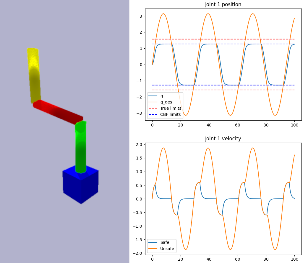
Manipulator Joint Limit Avoidance
Use a CBF to keep a manipulator operating within its joint limits, even if a nominal joint trajectory is unsafe.
- State: z = [Joint angles] (n = 3)
- Control: u = [Joint velocities] (m = 3)
- Relative degree: 1
Drone Obstacle Avoidance
Use a CBF to keep a drone inside a safe box, while avoiding a moving obstacle. This is similar to the "point robot obstacle avoidance" demo, but with slightly different dynamics.
- State: z = [Position, Velocity] (n = 6)
- Control: u = [Velocity] (m = 3)
- Relative degree: 1
- Additional data: The state of the obstacle (position and velocity)
This is the same CBF which was used in the "Drone Fencing" demo at the Stanford Robotics center.
Release history Release notifications | RSS feed


Download files
Download the file for your platform. If you're not sure which to choose, learn more about installing packages.
Source Distribution
Built Distribution
Filter files by name, interpreter, ABI, and platform.
If you're not sure about the file name format, learn more about wheel file names.
Copy a direct link to the current filters
File details
Details for the file cbfpy-0.0.3.tar.gz.
File metadata
- Download URL: cbfpy-0.0.3.tar.gz
- Upload date:
- Size: 36.8 kB
- Tags: Source
- Uploaded using Trusted Publishing? No
- Uploaded via: twine/6.2.0 CPython/3.12.3
File hashes
| Algorithm | Hash digest | |
|---|---|---|
| SHA256 |
7c352b6197958de48b0db8abf11208e68aef8f4bdb224be3192863545e823b22
|
|
| MD5 |
a681bdf52fa4ae45696a4a39c20229db
|
|
| BLAKE2b-256 |
f7f2a6e059d37e839c3ae9a353f494bb739f8a411e4720df046a9e7ff54a4f4b
|
File details
Details for the file cbfpy-0.0.3-py3-none-any.whl.
File metadata
- Download URL: cbfpy-0.0.3-py3-none-any.whl
- Upload date:
- Size: 47.3 kB
- Tags: Python 3
- Uploaded using Trusted Publishing? No
- Uploaded via: twine/6.2.0 CPython/3.12.3
File hashes
| Algorithm | Hash digest | |
|---|---|---|
| SHA256 |
f03b2d980e8bf7477208c51740cecace238a86573bc4a52038940eba3e2811fb
|
|
| MD5 |
ac8ece921850bad8de2a18942d4a8831
|
|
| BLAKE2b-256 |
2481fcd9990ecda99ec8d27d44fe0929a60cdd350b248820106879d1ac104b2c
|


