
CHAID Segmentation
A self-contained Python package for population segmentation using CHAID decision trees. You give it a KPI/target and a set of predictors; it auto-bins the continuous predictors, grows a CHAID tree, and hands back interpretable segments with an event rate (or mean), population, population share and lift — plus a static tree chart where each node is a population and each branch is a choice.
It is built for the workflow: "input a KPI, generate a tree, read off the
high/low segments of the customer base." For example, for a 90+DPD target:
age < 25 AND region = Phnom Penh AND bank = ABA → 60% 90+DPD rate, 10% of population, 2.5x lift
The CHAID tree engine is bundled in this repository — there is no external
CHAID dependency to install. It is based on the
Rambatino/CHAID project (Apache 2.0); see
Credits & License.
Features
- Automatic binning of continuous predictors — supervised (target-based), equal-width, equal-frequency (quantile) or manual cut points, chosen per variable.
- Binary and continuous KPIs — node rate is the event rate
P(target = positive)for a binary target, or the mean for a continuous target. - Interpretable segments — every terminal node becomes a readable rule with rate, population, population share and lift.
- Static visualisation (matplotlib + seaborn) — node = population, branch = choice, colour = rate.
- Predict / score new data by re-applying the fitted bins and rules.
- Load straight from CSV or Parquet with one call.
Installation
Requires Python 3.9+. Install from this repository:
pip install .                       # core (numpy, pandas, scipy, matplotlib, seaborn, ...)
pip install '.[segmenter-target]'   # + optbinning, for method="target" (supervised binning)
pip install '.[parquet]'            # + pyarrow, for ChaidSegmenter.from_parquet
matplotlib and seaborn are core dependencies (binning + plotting). optbinning
and pyarrow are only needed for target-based binning and Parquet loading
respectively, and are imported lazily with a clear error if missing.
How to use
import pandas as pd
from chaid_segmenter import ChaidSegmenter

df = pd.read_csv("loan_book.csv")     # columns: age, income, tenure, score, region, bank, dpd90

seg = ChaidSegmenter(
    target="dpd90",
    positive_class=1,                                    # binary event-rate target
    predictors={
        "age":    {"method": "target", "max_bins": 4},      # supervised (optbinning)
        "income": {"method": "equal_width", "bins": 4},     # fixed-interval bins
        "tenure": {"method": "equal_frequency", "bins": 4}, # quantile bins
        "score":  {"method": "manual", "edges": [550, 650, 750]},
        "region": {"method": "nominal"},                    # categorical, used as-is
        "bank":   {"method": "nominal"},
    },
    max_depth=3,
    min_child_node_size=0.02,         # int count, or a fraction of the dataset
    alpha_merge=0.05,
)
seg.fit(df)

seg.summary()                         # tidy DataFrame, highest rate first
seg.segments()                        # list[Segment]
seg.predict(df_new)                   # assign rows to terminal segments
seg.plot("tree.png")                  # static matplotlib/seaborn chart
seg.tree_frame()                      # raw tree, one row per node -- DataFrame
seg.tree_dict()                       # raw tree, nested dict -- for custom plots/graphs
Load and fit in a single call:
seg = ChaidSegmenter.from_csv("loan_book.csv", "dpd90", predictors, positive_class=1)
seg = ChaidSegmenter.from_parquet("loan_book.parquet", "dpd90", predictors, positive_class=1)
A runnable, self-contained demo lives at
examples/dpd_segmentation.py.
You don't have to spell out every predictor
predictors accepts three forms — pick whichever is least effort:
# 1. Full control: a spec (or method string) per column
predictors={"age": {"method": "target", "max_bins": 4}, "region": "nominal"}

# 2. Just the column names — the method is inferred from each column's dtype
#    (numeric -> default_numeric_method, non-numeric -> nominal)
predictors=["age", "income", "region", "bank"]

# 3. Omit it entirely — auto-select every column except the target/weight
ChaidSegmenter(target="dpd90", positive_class=1).fit(df)
In full-auto mode, constant columns and high-cardinality text columns (IDs, names,
free text — anything with more than max_nominal_cardinality distinct values) are
skipped automatically. You can always mix inference with overrides — e.g.
{"age": "auto", "score": {"method": "manual", "edges": [550, 650]}} — and inspect
what was chosen via seg.resolved_predictors after fit. Inferred numeric columns
use default_numeric_method (default "target", falling back gracefully if you
prefer "equal_frequency"/"equal_width").
Expected output
seg.summary()
A pandas.DataFrame, one row per terminal segment, highest rate first:
 node_id                                                           description population population_pct  rate  lift
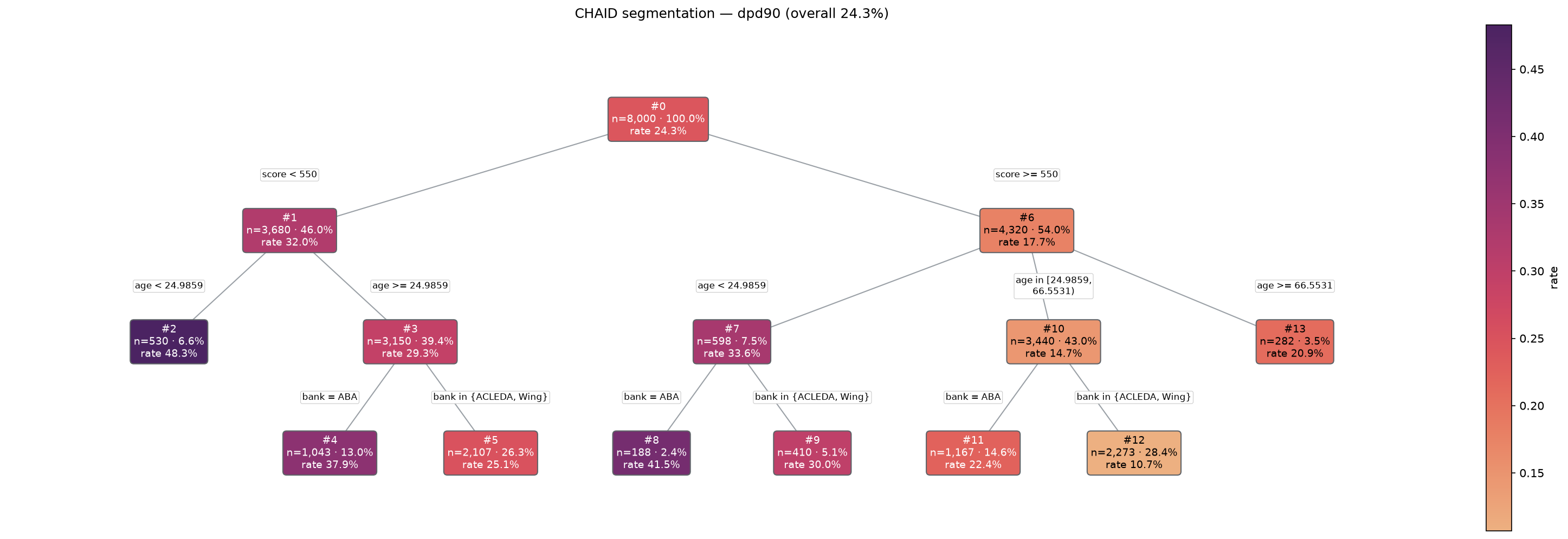
       2                                         age < 24.9859 AND score < 550        530           6.6% 48.3% 1.99x
       8                         bank = ABA AND age < 24.9859 AND score >= 550        188           2.4% 41.5% 1.71x
       4                         bank = ABA AND age >= 24.9859 AND score < 550      1,043          13.0% 37.9% 1.56x
       9             bank in {ACLEDA, Wing} AND age < 24.9859 AND score >= 550        410           5.1% 30.0% 1.24x
       5             bank in {ACLEDA, Wing} AND age >= 24.9859 AND score < 550      2,107          26.3% 25.1% 1.03x
      11             bank = ABA AND age in [24.9859, 66.5531) AND score >= 550      1,167          14.6% 22.4% 0.92x
      13                                       age >= 66.5531 AND score >= 550        282           3.5% 20.9% 0.86x
      12 bank in {ACLEDA, Wing} AND age in [24.9859, 66.5531) AND score >= 550      2,273          28.4% 10.7% 0.44x
seg.segments()
Each Segment is a small object you can read off directly:
top = seg.segments()[0]
top.description     # 'age < 24.9859 AND score < 550'
top.rate            # 0.4830...   (48.3% 90+DPD rate)
top.population      # 530.0
top.population_pct  # 0.06625     (6.6% of the book)
top.lift            # 1.99        (vs the 24.3% overall rate)
top.node_id         # 2
top.rules           # [{'variable': 'age', 'label': 'age < 24.9859', 'data': [...]},
                    #  {'variable': 'score', 'label': 'score < 550', 'data': [...]}]
seg.plot("tree.png")
Each node shows its population (count + % of total) and rate; each branch is labelled with the choice that leads into it; node colour encodes the rate:
seg.tree_frame() / seg.tree_dict()
Everything plot() draws, as data instead of a picture — one row/dict per
tree node (internal and terminal, not just the final segments), with the
same split variable, incoming-branch condition, population, rate, lift and
layout position (x, y) used to render the chart above. Use these to build
your own plot (Plotly, Graphviz, D3, NetworkX, ...):
>>> seg.tree_frame().head()
   node_id  parent_id  depth  is_terminal split_variable branch_variable    branch_label  population  population_pct   rate  lift   x    y  children
0        0       None      0        False            age           None            None      8000.0          1.0000 0.2430  1.00 3.5  0.0  [1, 2]
1        1          0      1         True           None            age       age < 25      1200.0          0.1500 0.4830  1.99 1.0 -1.0        []
2        2          0      1        False         score            age      age >= 25      6800.0          0.8500 0.2010  0.83 4.5 -1.0  [3, 4]

>>> seg.tree_dict()
{'node_id': 0, 'parent_id': None, 'split_variable': 'age', 'branch_label': None,
 'rate': 0.243, ..., 'children': [{'node_id': 1, 'branch_label': 'age < 25', ...}, ...]}
tree_dict() is plain nested dicts/lists (json.dumps-able), so it drops
straight into JSON-based/hierarchical viz libraries.
seg.predict(df, with_rate=True)
Assigns every row to its terminal segment (and, optionally, that segment's rate):
>>> seg.predict(df_new, with_rate=True).head()
   node_id      rate
0       11  0.223650
1        4  0.378715
2       12  0.106907
3        5  0.250593
4        4  0.378715
Rows that match no segment (e.g. an unseen category at predict time) come back as <NA>.
Binning methods
Each predictor's method selects how it is turned into branches:
method |
Spec keys | Description |
|---|---|---|
target |
max_bins |
Supervised optimal binning via optbinning — monotonic event rate. Works on numeric columns (rate-ordered ranges) and on high-cardinality categoricals (groups categories into rate tiers). Needs the segmenter-target extra. |
equal_width |
bins |
Fixed-width intervals across the value range. |
equal_frequency |
bins |
Quantile bins of roughly equal population. |
manual |
edges |
User-supplied interior cut points. |
nominal |
— | Categorical predictor, used as-is (no binning). |
Continuous predictors are converted to ordinal bin codes, so only contiguous
bins ever merge and every branch renders as a clean range (age < 25,
in [25, 40), >= 40). Missing values become their own missing branch.
A spec may be written as a bare method string when it takes no options, e.g.
"region": "nominal".
High-cardinality IDs (member / institution codes)
A categorical with hundreds of distinct values — a member id, institution code,
merchant id — can't be used as plain nominal (CHAID would try to merge hundreds
of categories: slow and unreadable). Use target to group it by the event rate
into a few risk tiers:
predictors={"MEMBER_ID": "target", "PRODUCT_TYPE": "nominal", ...}
Segments then read like MEMBER_ID in {003, 014, 019, 024, 045, 048, +11} → 40.7%
— a concrete high-risk member group. This also happens automatically when you simply
list such a column (its cardinality exceeds max_nominal_cardinality); in
full-auto mode (predictors omitted) high-cardinality columns are dropped instead,
since the tool can't tell a meaningful id from a row identifier like ACCOUNT_ID.
Numeric-looking ids. Whether a column is binned as a number or grouped as a category is decided from its dtype. An id like
001..200read from a CSV becomesint64, so it would be binned into meaningless ranges (MEMBER_ID < 100). Either cast it to text —df["MEMBER_ID"] = df["MEMBER_ID"].astype(str)(or read withpd.read_csv(..., dtype={"MEMBER_ID": str})) — or force grouping with{"method": "target", "categorical": True}.
Targets
- Binary — pass
positive_class(the event value, e.g.1). NoderateisP(target == positive_class)andliftisrate / overall_rate. - Continuous — omit
positive_class. Noderateis the mean of the target andliftismean / overall_mean.
API reference
ChaidSegmenter(...)
| Parameter | Default | Description |
|---|---|---|
target |
— | Name of the KPI/target column. |
predictors |
None |
A {column: spec} dict, a list of column names (methods inferred from dtype), or None for full auto-select. See Binning methods and above. |
positive_class |
None |
Event value for a binary target; None ⇒ continuous target. |
default_numeric_method |
"target" |
Binning method for auto-inferred numeric predictors (target / equal_frequency / equal_width). |
default_bins |
5 |
Bin count for auto-inferred numeric predictors. |
max_nominal_cardinality |
20 |
In full-auto mode, non-numeric columns with more distinct values are skipped. |
max_depth |
3 |
Maximum tree depth. |
min_child_node_size |
30 |
Minimum observations per child. Values in (0, 1) are treated as fractions of the dataset. |
min_parent_node_size |
None |
Minimum observations to split a node; defaults to min_child_node_size. Fractions supported. |
alpha_merge |
0.05 |
Significance threshold for merging predictor categories. |
split_threshold |
0 |
Surrogate-split threshold (passed through to the tree engine). |
max_splits |
None |
Maximum number of children per split. |
weight |
None |
Optional weight column; populations and rates use weighted sums. |
Methods
fit(df)— fit the binners and grow the tree from apandas.DataFrame.segments(sort_by_rate=True)— list ofSegmentobjects.summary()— segments as a tidyDataFrame.segment_rates—{node_id: rate}for the terminal nodes.predict(df, with_rate=False)— terminalnode_idper row (optionally with rate).plot(path=None, **kwargs)— render the tree; returns(fig, layout)and writes topathif given. Acceptsfigsize,cmap,dpi, font-size overrides.tree_frame()— every tree node (not just terminals) as a tidyDataFrame, for building a custom plot/graph of the tree.tree_dict()— the tree as a nesteddict(root →children→ ...), for hierarchical/JSON-based plotting libraries.ChaidSegmenter.from_csv(path, target, predictors, *, read_csv_kwargs=None, **kwargs)andfrom_parquet(...)— load a file, construct andfitin one call.
Segment
node_id, description, rate, population, population_pct, lift, and a
structured rules list of {variable, label, data}.
How it works
ChaidSegmenter fits a Binner per continuous predictor and feeds the resulting
integer bin codes (as ordinal columns) plus the nominal predictors into a
bundled CHAID tree engine, which splits on the predictor most strongly associated
with the target (chi-squared for categorical targets, Bartlett's/Levene's test for
continuous targets). Because the bins enter as contiguous ordinal codes, merged
groups always describe a single, readable range. Terminal nodes are then translated
back into rate/population/lift segments.
Low-level tree engine
The underlying CHAID tree implementation is bundled and importable as CHAID
(from CHAID import Tree) for advanced use — building a tree by hand, exporting
classification_rules(), treelib conversion, etc. The segmentation API above is the
recommended entry point for the KPI-segmentation workflow.
Testing
pip install -e '.[segmenter-target,parquet,test]'
pytest tests/
Credits & License
This project is built on top of CHAID
by Mark Ramotowski, Richard Fitzgerald and contributors. The CHAID/ package in
this repository is that upstream implementation, bundled unmodified as the
underlying tree engine. The chaid_segmenter/ package — automatic binning, KPI
segmentation and the matplotlib/seaborn visualisation — is an original addition.
Distributed under the Apache License 2.0. See LICENSE.txt for the full license text and NOTICE for attribution.
1 maintainer

Metadata
1 maintainer
Release files for chaid-segmenter 1.0.1
For a detailed explanation of source distributions (sdists) and built distributions (wheels), please see the package formats documentation.
Source distribution (sdist)
| File | Size | Uploaded | |
|---|---|---|---|
| chaid_segmenter-1.0.1.tar.gz | 66.9 kB | Details |
Built distribution (wheel)
| File | Interpreter | ABI | Platform | Reset |
|---|---|---|---|---|
| chaid_segmenter-1.0.1-py3-none-any.whl | Python 3 | none | any | Details |
Total release size: 113.9 kB
Release files / chaid_segmenter-1.0.1.tar.gz
| Download URL | chaid_segmenter-1.0.1.tar.gz |
|---|---|
| Size | 66.9 kB |
| Tags | Source |
|
SHA-256 checksum How to use checksums |
2124407c0aa510507ea79eb4d06d66dbf5d2b0ad9528387fed92983d3f55362b
|
|
BLAKE2b-256 checksum How to use checksums |
e9c5ef9424654ba879a085f9c9f621b0362299ca8604dc74a978597866c8e778
|
| Upload date | |
|
Uploaded using Trusted Publishing? What is trusted publishing? |
No |
| Uploaded via |
twine/7.0.0 CPython/3.12.3
|
Release files / chaid_segmenter-1.0.1-py3-none-any.whl
| Download URL | chaid_segmenter-1.0.1-py3-none-any.whl |
|---|---|
| Size | 47.0 kB |
| Tags | Python 3 |
|
SHA-256 checksum How to use checksums |
ae5df1ff5f6b75a56281579258142c39e86286619474cc66b3994de460eed23a
|
|
BLAKE2b-256 checksum How to use checksums |
86b0f6faf67e413f324eb5dea91de373b6425bcc05bd87dc279d64df88ccdb99
|
| Upload date | |
|
Uploaded using Trusted Publishing? What is trusted publishing? |
No |
| Uploaded via |
twine/7.0.0 CPython/3.12.3
|














