
ChEBI-N
ChEBI-N is an updated version of BiNChE. It is a tool for ontology-based chemical enrichment analysis and uses the ChEBI ontology of chemical entities as its background population.
It is available both as the chebin Python package and as a web application at
https://chebin.hastingslab.org/ that needs no local setup.
Package usage
Installation
ChEBI-N is published on PyPI as chebin and
requires Python 3.12 or newer:
pip install chebin
or, with uv:
uv add chebin
Installing from a local build instead (for development)
To work against your own checkout rather than the released package, build a wheel and point another project at it:
cd chebin
uv build
This produces dist/chebin-<version>-py3-none-any.whl. Point another project at
it:
- With
uv, add to yourpyproject.toml:[project] dependencies = ["chebin"] [tool.uv.sources] chebin = { path = "/path/to/chebin/dist/chebin-<version>-py3-none-any.whl" }
then runuv sync. - With plain
pip:pip install /path/to/chebin/dist/chebin-<version>-py3-none-any.whl.
Whenever the source changes, rebuild the wheel (uv build) and re-sync to pick it
up. With uv, that's uv lock --upgrade-package chebin && uv sync --- the wheel
is pinned in uv.lock by exact file hash, so a same-version rebuild isn't picked
up automatically otherwise.
Step 1: Generate the data files (required first)
Every function below needs a generated data folder. Build one with:
from chebin import create_all_files

create_all_files(data_folder="data")
This can take up to a few hours --- it downloads and processes the full ChEBI ontology, LOTUS/Wikidata compound data, and the Recon3D model. It only needs to be run once (re-run it later to refresh with newer ChEBI/LOTUS data).
Before running the function, one input has to be supplied by hand:
hmdb_metabolites.xml (the 'All Metabolites' export from
HMDB), placed in data/ or data/source_files/.
Without it, create_all_files still runs and prints a warning, but skips the
broad Homo sapiens background (HMDB + LOTUS) and everything that depends on it.
Once it finishes, data_folder (data/ by default) holds everything the
enrichment functions read directly; the source_files/ and
intermediate_files/ subfolders it also creates are working files nothing reads
afterwards --- safe to delete (each has its own README explaining what it is).
If you're regenerating an existing data folder rather than building one from
scratch, use create_all_files_with_backup instead --- it isn't re-exported at
the top level, so import it directly:
from chebin.preparing_data.create_files import create_all_files_with_backup

create_all_files_with_backup(data_folder="data")
This renames the current data/ to data_last_used_YYYY.MM.DD before building
the replacement, and keeps only the 3 most recent backups.
Note that chebin looks for the data folder at
<current working directory>/data, so run your analyses from the folder you
generated it in. If that isn't possible, point chebin at it with
set_data_dir("/path/to/data") or the CHEBIN_DATA_DIR environment variable.
See the Datafiles Workflow section below for a step-by-step breakdown of what each stage does and what each file consists of.
Enrichment analysis functions
Different functions are provided for different combinations of options. For the simplest usage, skip ahead to the example below.
All functions follow one naming pattern:
run_[weighted_][narrow_background_]enrichment_analysis[_plain_enrich_pruning_strategy][_from_smiles]
Wherever these functions take a ChEBI ID --- in studyset_list, as a
weights_dict key, or as a seed elsewhere --- it is recognised however it is
written: CHEBI:17079, chebi:17079, ChEBI:17079, CHEBI_17079,
CHEBI 17079, CHEBI ID: 17079, the bare number 17079 and the full IRI
http://purl.obolibrary.org/obo/CHEBI_17079 all mean the same entity. Note that
each ID must be its own list element or dict key: "17079 17080" is one
(meaningless) entry rather than two entities.
Four independent choices combine to give the full name:
-
weighted_--- plain Fisher's exact test (unweighted) vs. the SaddleSum-derived weighted method (see Calculations). Unweighted functions takestudyset_list(a list of ChEBI IDs); weighted functions takeweights_dict(ChEBI ID -> weight, all weights must be real and positive), written as a plain dict:weights_dict = {"CHEBI:15377": 1.5, "CHEBI:16236": 0.8, "CHEBI:17234": 3.0} results, graph = run_weighted_enrichment_analysis(weights_dict)
The
_from_smilesweighted variants take the same shape with structure keys instead (a{SMILES or InChI: weight}dict), e.g.{"CC(=O)Oc1ccccc1C(=O)O": 1.5, "CHEBI:16236": 0.8}--- SMILES, InChI and ChEBI ID keys can be mixed freely. -
narrow_background_--- the whole ChEBI ontology as background vs. a restricted background (see Background). Choose which by passingnarrow_background_leaves_json:Background narrow_background_leaves_jsonHomo sapiens broad (LOTUS + HMDB) --- default "human"Homo sapiens narrow (Recon3D) "endogenous_human"Arabidopsis thaliana "arabidopsis_thaliana"An explicit path to a leaves JSON also still works (e.g. a custom background for another taxon) --- the three short names above are just a convenience for the built-in ones:
results, graph, leaves, parents = run_narrow_background_enrichment_analysis(
    ["CHEBI:15377", "CHEBI:16236"],
    narrow_background_leaves_json="data/my_taxon_leaves.json",
)
The only key read from that file is
"narrow_leaves", listing the background's leaf classes as ChEBI IRIs. The generated files carry provenance keys alongside it (taxon_label,compounds_tsv, ...), but those are ignored here, so a hand-written background only needs:{ "narrow_leaves": [ "http://purl.obolibrary.org/obo/CHEBI_10038", "http://purl.obolibrary.org/obo/CHEBI_10043" ] }
expand_background(defaultTrue) controls what happens to study-set compounds outside the chosen background: kept and added to the background too (so every input still gets tested) ifTrue, excluded from the study set entirely ifFalse. The two extra return values,leaves_to_expand_background/parents_to_expand_background, report which leaves/input classes triggered that expansion either way. -
_plain_enrich_pruning_strategy--- the fixed Plain Enrichment Pruning Strategy vs. manually choosing which pruners to apply and when. -
_from_smiles--- takes structures instead of ChEBI IDs (alist[str]of SMILES and/or InChI, or{SMILES or InChI: weight}for weighted variants), resolved to ChEBI ID(s) the same way described in Study Set, plus ause_parents: bool = Falseparameter (fall back to predicted parent classes when a structure has no direct ChEBI match if set toTrue). An input is read as an InChI when it starts withInChI=, and as a SMILES otherwise. Returns everything the ChEBI-ID version does, plus one extra dict:{"unresolved_smiles": [...], "ambiguous_matches": [...], "invalid_structures": [...]}.unresolved_smilesis the plain list of inputs that resolved to no ChEBI class at all.invalid_structuresis the subset of those that RDKit could not read as a molecule in the first place. These are reported but dropped. An ambiguous match is the opposite problem --- a structure that matched several ChEBI classes at once. Only one of them enters the study set (the lowest ChEBI ID, so the same input always resolves the same way), and the runners-up are reported here rather than silently dropped:{"smiles": "CCO", "chosen": "CHEBI:16236", "alternatives": ["CHEBI:17246"]}
so you can check whether the chosen class was the one you meant. This list is usually short, but worth a glance. A mixture of SMILES, InChI and ChEBI IDs can be used. Both the
_smilessuffix and the"smiles"key predate InChI support and are kept for compatibility; each reports whichever form was submitted, so an InChI input is echoed back as the InChI string you passed in, not as the SMILES it was converted to.
The table below shows all the different types of enrichment analysis functions. The "manual" rows take the individual pruner toggles as ordinary arguments --- see Shared parameters for the full list, and the manual-pruning example below for what a call looks like. Rows whose input is listed as "SMILES" accept InChI in the same argument, and either may be mixed with ChEBI IDs.
| Function | Input | Background | Pruning | Returns |
|---|---|---|---|---|
run_enrichment_analysis |
ChEBI IDs + pruning options | whole ontology | manual | (results, graph) |
run_enrichment_analysis_plain_enrich_pruning_strategy |
ChEBI IDs | whole ontology | plain strategy | (results, graph) |
run_enrichment_analysis_from_smiles |
SMILES + pruning options | whole ontology | manual | (results, graph, smiles_diagnostics) |
run_enrichment_analysis_plain_enrich_pruning_strategy_from_smiles |
SMILES | whole ontology | plain strategy | (results, graph, smiles_diagnostics) |
run_weighted_enrichment_analysis |
ChEBI IDs + weights + pruning options | whole ontology | manual | (results, graph) |
run_weighted_enrichment_analysis_plain_enrich_pruning_strategy |
ChEBI IDs + weights | whole ontology | plain strategy | (results, graph) |
run_weighted_enrichment_analysis_from_smiles |
SMILES + weights + pruning options | whole ontology | manual | (results, graph, smiles_diagnostics) |
run_weighted_enrichment_analysis_plain_enrich_pruning_strategy_from_smiles |
SMILES + weights | whole ontology | plain strategy | (results, graph, smiles_diagnostics) |
run_narrow_background_enrichment_analysis |
ChEBI IDs + pruning options | restricted | manual | (results, graph, leaves_to_expand_background, parents_to_expand_background) |
run_narrow_background_enrichment_analysis_plain_enrich_pruning_strategy |
ChEBI IDs | restricted | plain strategy | (results, graph, leaves_to_expand_background, parents_to_expand_background) |
run_narrow_background_enrichment_analysis_from_smiles |
SMILES + pruning options | restricted | manual | (results, graph, leaves_to_expand_background, parents_to_expand_background, smiles_diagnostics) |
run_narrow_background_enrichment_analysis_plain_enrich_pruning_strategy_from_smiles |
SMILES | restricted | plain strategy | (results, graph, leaves_to_expand_background, parents_to_expand_background, smiles_diagnostics) |
run_weighted_narrow_background_enrichment_analysis |
ChEBI IDs + weights + pruning options | restricted | manual | (results, graph, leaves_to_expand_background, parents_to_expand_background) |
run_weighted_narrow_background_enrichment_analysis_plain_enrich_pruning_strategy |
ChEBI IDs + weights | restricted | plain strategy | (results, graph, leaves_to_expand_background, parents_to_expand_background) |
run_weighted_narrow_background_enrichment_analysis_from_smiles |
SMILES + weights + pruning options | restricted | manual | (results, graph, leaves_to_expand_background, parents_to_expand_background, smiles_diagnostics) |
run_weighted_narrow_background_enrichment_analysis_plain_enrich_pruning_strategy_from_smiles |
SMILES + weights | restricted | plain strategy | (results, graph, leaves_to_expand_background, parents_to_expand_background, smiles_diagnostics) |
All are importable directly from chebin, e.g.
from chebin import run_weighted_narrow_background_enrichment_analysis_from_smiles.
Shared parameters
These appear on most or all of the functions above (see the linked sections for what each option means):
| Parameter | Default | Meaning |
|---|---|---|
bonferroni_correct |
False |
Apply Bonferroni correction (Correction Method) |
benjamini_hochberg_correct |
True |
Apply Benjamini-Hochberg FDR correction (overrides Bonferroni if both are True) |
root_children_prune |
False |
Apply the Root Children Pruner |
levels |
2 |
Levels pruned by the Root Children Pruner |
linear_branch_prune |
False |
Apply the Linear Branch Collapser Pruner |
n |
2 (manual) / 0 (plain strategy) |
Keep every n-th node along a linear branch (Linear Branch Collapser Pruner); n = 0 removes every intermediate node, so a larger n prunes more and n = 1 prunes nothing |
high_p_value_prune |
False |
Apply the High P-Value Branch Pruner |
p_value_threshold |
0.05 |
Threshold used by the High P-Value Branch Pruner |
zero_degree_prune |
False |
Apply the Zero-degree Pruner |
classification |
"structural" |
Which part of the ontology to run on: "structural", "functional", or "full" (see Background) |
print_results |
False |
Print a p-value table to stdout |
csv_output_path |
None |
If given, write the results table to this CSV path |
The _plain_enrich_pruning_strategy functions don't take the individual
*_prune toggles --- the plain strategy always applies its fixed pruner
sequence --- but still take levels, n, and p_value_threshold to tune it.
Visualisation
export_graph_html(G, enrichment_results, output_file, include_untested_leaves=False)
Writes G (the graph returned by any run_* function above) as a
self-contained interactive HTML page --- no server or network access needed to
view it. enrichment_results is the results dict returned alongside G; pass
None if you don't have one (the graph still renders, just without p-values or
colouring). include_untested_leaves is off by default: study-set leaves are
never tested (so never coloured) and are typically the large majority of nodes,
so including them mostly just slows down rendering --- set it to True to keep
them anyway, e.g. for debugging.
Step 2: Quick example (run an analysis, then export the graph)
from chebin import run_enrichment_analysis_plain_enrich_pruning_strategy, export_graph_html

results, graph = run_enrichment_analysis_plain_enrich_pruning_strategy(
    ["CHEBI:15377", "CHEBI:16236", "CHEBI:17234"],
    print_results=True,             # print a p-value table to stdout
    csv_output_path="results.csv",  # and write it to CSV
)

export_graph_html(graph, results, "enrichment_graph.html")
To choose the pruners yourself instead, call the function without
_plain_enrich_pruning_strategy and switch them on individually:
from chebin import run_enrichment_analysis, export_graph_html

results, graph = run_enrichment_analysis(
    ["CHEBI:15377", "CHEBI:16236", "CHEBI:17234"],
    high_p_value_prune=True,   # drop branches with no significant node ...
    p_value_threshold=0.05,    #   ... using this threshold
    linear_branch_prune=True,  # collapse unbranched chains ...
    n=2,                       #   ... keeping every 2nd node (n=0 removes all)
    root_children_prune=True,  # drop the most general classes ...
    levels=2,                  #   ... the roots plus 1 level of descendants
    zero_degree_prune=True,    # drop nodes left unconnected by the above
    classification="full",     # structure + role hierarchies
)

export_graph_html(graph, results, "enrichment_graph.html")
Every pruner is off by default, so passing none of them runs the enrichment and returns the graph unpruned. Manually chosen pruners are applied once each, in contrast to the plain strategy, which loops until no further nodes are removed (see Pruning Strategies).
results is a dict with "study_set" (input names), "removed_nodes" (names
of nodes pruned away), and "enrichment_results" (class name -> p-value
details). graph is the pruned networkx graph, ready to hand to
export_graph_html, which writes a self-contained interactive HTML page --- no
server or network access needed to view it.
The Web Application
The web application is available at https://chebin.hastingslab.org/. It offers the same analyses as the package, without any local setup.
Running The Analysis
To run calculations locally instead, execute website/app.py in the repository.
Note that all necessary data files must be generated beforehand for local
execution --- either as described in the Datafiles
Workflow section below, or using the package as described
above.
Study Set
On the home page, you can enter your study set as ChEBI IDs (one per line), SMILES or InChI. You can optionally provide weights for each compound (tab- or space-separated).
Entities can be separated by a new line, a comma, a space or a tab, and these
can be mixed freely (CHEBI:17079, CHEBI:46816 on one line and CHEBI:31463 on
the next is three entities). The one exception is InChI, which contains commas
of its own: an InChI has to be separated by a new line, a space or a tab, since
a comma-separated InChI would be read as several entities. When submitting
weights, give each entity its own line: the weight is taken from the second
column, so any further entries on the same line are ignored.
ChEBI IDs are recognised however they are written, so a list copied from another
tool does not have to be reformatted first: CHEBI:17079, chebi:17079,
ChEBI:17079, CHEBI_17079, CHEBI 17079, CHEBI ID: 17079, the bare number
17079 and the full IRI http://purl.obolibrary.org/obo/CHEBI_17079 all mean
the same entity. The same applies to the ChEBI IDs passed to the enrichment
analysis functions directly. One caveat for
weights: since a bare number is a valid ID, a whole number in the second column
of a line whose ID is also a bare number is read as a second ID rather than a
weight (17079 17080 is two entities). Write the weight as a decimal, or prefix
the ID with CHEBI:, to submit weights.
An input starting with InChI= is read as an InChI and parsed into a molecule
first; every step below then works from that molecule, so SMILES and InChI share
one resolution path and the same input structure resolves identically whichever
form it was written in. A bare InChIKey is not accepted --- it is a hash with no
recoverable structure, so there is nothing to parse or look up a canonical form
for.
If SMILES or InChI are used, each structure is resolved to a ChEBI ID in this order: (1) an exact string match against the local table of ChEBI leaf classes, (2) a match via the InChIKey computed from the structure, (3) a direct lookup through the Chebifier API. If none of these resolve, its predicted direct parent classes (also from Chebifier) can optionally be used for enrichment calculations instead. The Chebifier API accepts SMILES only, so an InChI is sent as the canonical SMILES it was parsed into. Where a structure matches several ChEBI entries, only one of them is included in the analysis (the lowest ChEBI ID); the alternatives are listed on the results page as ambiguous matches. Note that this applies to a structure matching several ChEBI terms --- where a structure is instead resolved to its predicted parent classes, all of those parents are included.
When a parent class is included in the study set, it is replaced by all of its leaf descendants.
Background
Using the whole ChEBI ontology as a background population is the standard option; alternatively, only the 'Structure' or 'Role' hierarchy can be used as the target of enrichment:
- Structure: Enrichment based on ChEBI structural classification. This target is based on classes descending from the root node 'chemical entity', filtered to include everything under its children 'chemical substance' and 'molecular entity' (and not under 'atom' and 'group').
- Role: Enrichment based on ChEBI role classification. This is based on classes descending from the root node 'role'.
- Both: Union of structure and role classifications (note that the structure classification is significantly larger).
(In the package these are the classification argument: Structure is
"structural" (the default), Role is "functional", and Both is
"full".)
A restricted, more specific background can also be used. For each restricted background, a set of leaf classes is specified using external sources, as explained below. All the ancestor classes of those leaves in the ChEBI ontology then form the background population, so only a subset of the ontology is used.
Human background - broad (LOTUS and HMDB)
Compounds from HMDB and LOTUS (taxonomy = Homo sapiens) were mapped to ChEBI leaf classes to serve as a background for enrichment. These are entities that have been measured from human samples.
Matching to a ChEBI ID was attempted in this order: (1) a ChEBI ID already present in the source data, (2) an exact SMILES match against the local table of ChEBI leaf classes (Wikidata only), (3) an InChIKey lookup against the same local table, (4) the Chebifier API, which performs both a direct lookup and parent-class classification, keeping all of the direct parent classes it returns.
Where the steps above left an entity with more than one ChEBI ID --- from any of them, not just the Chebifier parents --- only the deepest were kept, to avoid overly broad annotations. "Deepest" here means the longest path to a root of the ChEBI hierarchy, i.e. this should represent the most specific class. Where a matched ChEBI ID corresponded to a non-leaf class in the ontology, it was expanded to its leaf descendants; classes with more than 150 leaf descendants were excluded to prevent high-level classes from disproportionately inflating the background. The resulting set of leaf classes was used to form the restricted background for the enrichment analysis.
Human background - narrow (Recon3D)
A second, narrower human background was built from Recon3D, a genome-scale reconstruction of human metabolism, downloaded as JSON from BiGG Models. Unlike the Human background above, this one is restricted to metabolites that participate in modelled human metabolic reactions, so it excludes externally sourced human-associated compounds (e.g. drugs, diet).
Recon3D represents each metabolite once per cellular compartment it appears in
(e.g. 10fthf_c, 10fthf_m for the cytosolic and mitochondrial pools of the
same compound), so compartment-specific entries sharing a base BiGG ID were
first collapsed into a single compound record --- these always carry identical
formula, charge, and database cross-references, confirming they are the same
chemical species. This reduced Recon3D's 5,835 metabolite entries to 2,797
unique compounds.
Each compound's listed ChEBI ID(s) were then resolved to leaf classes as follows:
- If any listed ChEBI ID is already a leaf, all such leaf candidates were kept. BiGG often lists several ChEBI IDs for one compound (e.g. different protonation or tautomer states), and these are typically genuinely distinct structures rather than duplicates, so none were discarded in favour of a single "primary" one.
- If none of the listed IDs is a leaf, each was expanded to its leaf descendants, excluding any class with more than 150 leaf descendants (the same cutoff used for the Human background, to avoid over-generic classes).
- For compounds with no ChEBI annotation at all, a ChEBI cross-reference was attempted via UniChem, first by InChIKey, then by HMDB ID (Recon3D stores HMDB IDs in an older 5-digit format, which was zero-padded to UniChem's expected 7-digit format before lookup). Any ChEBI IDs found this way were resolved to leaves using rules 1--2 above.
Compounds for which none of the above resolved to a leaf were left out of the background.
Arabidopsis thaliana Background
This background also uses data from LOTUS but with taxonomy = Arabidopsis thaliana. Mapping was done in the same way as for the broad human background.
Correction Method
For multiple hypothesis testing correction, p-value correction methods are available. The options are Benjamini-Hochberg, Bonferroni, and None. Benjamini-Hochberg is generally recommended.
Bonferroni is the simplest method: the corrected p-value is obtained by multiplying the original p-value by the number of separate tests performed.
Benjamini-Hochberg instead controls the false discovery rate, by exploiting the fact that p-values are uniformly distributed under the null hypothesis. The p-values are sorted in ascending order and each is divided by its rank to give a candidate adjusted value. To guarantee that adjusted p-values remain monotonic with rank, each value is then replaced by the minimum of itself and all candidate values computed for the less significant (higher-ranked) p-values.
Pruning Strategies
Pruning options are available to make the graph less cluttered. The following pruners are available:
-
Root Children Pruner: Removes the roots and their children up to a defined level (number of levels being an adaptable parameter). This allows removal of more general, and less meaningful, entities in the ontology. For example, levels set to 2 will remove the roots and one level of their descendants.
-
Linear Branch Collapser Pruner: Removes linear branches within the graph; only nodes with one parent and one child can be removed. Either a chosen number of nodes (n) in the linear branch will be kept, or all intermediate nodes in the branch can be removed (set n = 0). E.g., n = 3 will keep every third node in the branch.
Note that this pruner selects nodes by graph topology alone and does not consider p-values: an intermediate node is removed because of its position in a chain, regardless of how significant it is.
-
High P-Value Branch Pruner: Removes branches from the graph that only contain nodes with a p-value greater than 0.05 (this value can be changed). A node with a higher p-value will still be kept if it has at least one descendant with a p-value lower than the threshold.
-
Zero-degree Pruner: Removes nodes that have no connections with other nodes; that is, nodes with a total degree of zero.
If you manually choose which pruning strategies to apply, they will be implemented once each. Alternatively, pruning strategies can be implemented in a looping manner. In this scenario, there is first a pre-loop phase where pruners are applied once, and then a loop phase where pruners are applied in a loop until no more changes are made. The looping option is:
- Plain Enrichment Pruning Strategy: The pre-loop phase applies the high p-value branch pruner (with a threshold of 0.05), the linear branch collapser pruner (with n = 0), and the root children pruner (levels = 2). The loop phase applies the high p-value branch pruner (with a threshold of 0.05), the branch collapser pruner and the zero-degree vertex pruner. Benjamini-Hochberg is used as the p-value correction method, and is recomputed over the surviving classes on each loop iteration.
Calculations
Enrichment analysis uses Fisher's exact test for p-value calculations. For weighted enrichment analysis, however, a SaddleSum method is used. All weights must be real and positive numbers.
The SaddleSum implementation is largely based on SaddleSum-standalone-1.2.2.tar.gz, from https://ftp.ncbi.nlm.nih.gov/pub/qmbpmn/SaddleSum/src/. The code was translated from C to Python.
After the calculations have been carried out, a table of the raw and corrected p-values is provided. Below the table, further information is available --- for example, which nodes were removed by pruning.
The Graph
On the next webpage, a graph based on the enrichment analysis is displayed. The colouring of the nodes is based on the significance of the p-values, on a $-\log_{10}(p)$ scale. The corrected p-value is used for the colouring if it is available. Two colour scales can be chosen in the graph legend:
- Relative (default): the darkest colour is the smallest p-value in that graph. This makes the most of the colour range within one analysis, but colours cannot be compared between graphs.
- Absolute: the darkest colour is a fixed p-value cutoff (p ≤ 1e-x, where x is set next to the selector, 4 by default). Makes comparisons easier.
The graph will initially show only the most relevant branches. This means that all nodes with p-values under or equal to 0.05 will be shown, including all nodes in the paths from these nodes up to the root. If all nodes have a higher p-value, the same is done for nodes with p-values lower than 1. If every node has a p-value of 1 or N/A, all nodes are shown.
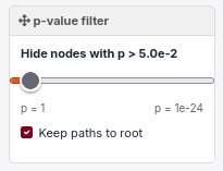
There is a slider with a p-value pruner making it possible to more precisely adapt what significance to show on the graph. Either paths to the root of nodes of the chosen p-value will be kept (even if their p-value is higher) or nodes will just be looked at individually. The second option will keep only the nodes with the chosen significance but may give 'island' nodes that are not connected to anything else. This slider is particularly useful for large datasets. The range of the slider is relative to the values obtained in that analysis. It can look like this:
There are options to choose the layout of the graph, which nodes are shown, and how to export the graph.
Re-running all calculations with new settings, such as with different pruning options, can be done by clicking on 'Settings'. The previously used options will be pre-selected.
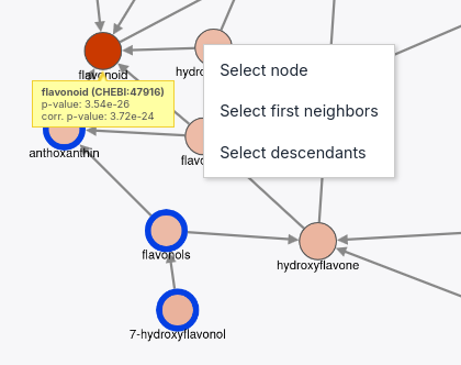
Hovering over a node displays more detailed information about it. Both raw and corrected p-values are shown, as well as its ChEBI ID. Clicking on the ID, or double-clicking on the node, will take you to that class' page on the ChEBI website.
Nodes can be selected by clicking on them. Right-clicking on a node provides the options as seen in the figure below.
Nodes can be repositioned by clicking and dragging them.
Leaf classes are not shown in the graph, since they do not receive p-values. Beyond the initial display described above, nodes can also be shown or hidden manually: options are available to hide all insignificant nodes (p-value > 0.05), to show all nodes, or to show/hide only the currently selected ones.
Datafiles Workflow
The data files the analysis reads are generated by create_all_files(), as
described under Generate the data
files above.
For a stage-by-stage breakdown of how each file is produced --- which script runs when, what it downloads, and what it writes --- see DATA_WORKFLOW.md.
1 maintainer

Metadata
1 maintainer
Release files for chebin 1.1.0
For a detailed explanation of source distributions (sdists) and built distributions (wheels), please see the package formats documentation.
Source distribution (sdist)
| File | Size | Uploaded | |
|---|---|---|---|
| chebin-1.1.0.tar.gz | 246.5 kB | Details |
Built distribution (wheel)
| File | Interpreter | ABI | Platform | Reset |
|---|---|---|---|---|
| chebin-1.1.0-py3-none-any.whl | Python 3 | none | any | Details |
Total release size: 498.8 kB
Release files / chebin-1.1.0.tar.gz
| Download URL | chebin-1.1.0.tar.gz |
|---|---|
| Size | 246.5 kB |
| Tags | Source |
|
SHA-256 checksum How to use checksums |
a914c79185dec0dc9ec4b9d6ab1dfc3e8f35d1e51743f9b499e6b3de51afa2d7
|
|
BLAKE2b-256 checksum How to use checksums |
8891a8b927725d149be0801349794f8104426ebfa8b7f76a554c1b4e71a0b9ff
|
| Upload date | |
|
Uploaded using Trusted Publishing? What is trusted publishing? |
Yes |
| Uploaded via |
uv/0.12.24 {"installer":{"name":"uv","version":"0.12.24","subcommand":["publish"]},"python":null,"implementation":{"name":null,"version":null},"distro":{"name":"Ubuntu","version":"24.04","id":"noble","libc":null},"system":{"name":null,"release":null},"cpu":null,"openssl_version":null,"setuptools_version":null,"rustc_version":null,"ci":true}
|
Provenance
Provenance describes where a file came from. On PyPI, provenance is shared via attestations, which provide a verifiable record of the build or publishing details. View details, limitations and caveats.


PyPI Publish Attestation
PyPI verified that this artifact, at this checksum, originated from the publisher listed below.
Signed by GitHub Actions, verified by PyPI on Oct 9, 2026.
Transparency logRelease files / chebin-1.1.0-py3-none-any.whl
| Download URL | chebin-1.1.0-py3-none-any.whl |
|---|---|
| Size | 252.3 kB |
| Tags | Python 3 |
|
SHA-256 checksum How to use checksums |
5ef347acaab10702b5afbec4e5430220d97dc789b3d8b5fc5d5371f10b6c7901
|
|
BLAKE2b-256 checksum How to use checksums |
7a7a9d269ef05a0a9975450d2a9e47442b211d85425403dc12b5cad481664f27
|
| Upload date | |
|
Uploaded using Trusted Publishing? What is trusted publishing? |
Yes |
| Uploaded via |
uv/0.12.24 {"installer":{"name":"uv","version":"0.12.24","subcommand":["publish"]},"python":null,"implementation":{"name":null,"version":null},"distro":{"name":"Ubuntu","version":"24.04","id":"noble","libc":null},"system":{"name":null,"release":null},"cpu":null,"openssl_version":null,"setuptools_version":null,"rustc_version":null,"ci":true}
|
Provenance
Provenance describes where a file came from. On PyPI, provenance is shared via attestations, which provide a verifiable record of the build or publishing details. View details, limitations and caveats.
PyPI Publish Attestation
PyPI verified that this artifact, at this checksum, originated from the publisher listed below.
Signed by GitHub Actions, verified by PyPI on Oct 9, 2026.
Transparency log













