Molecular Property Prediction with Message Passing Neural Networks


Project description
Molecular Property Prediction


This repository contains message passing neural networks for molecular property prediction as described in the paper Analyzing Learned Molecular Representations for Property Prediction and as used in the paper A Deep Learning Approach to Antibiotic Discovery.
Documentation: Full documentation of Chemprop is available at https://chemprop.readthedocs.io/en/latest/.
Website: A web prediction interface with some trained Chemprop models is available at chemprop.csail.mit.edu.
Tutorial: These slides provide a Chemprop tutorial and highlight recent additions as of April 28th, 2020.
COVID-19 Update
Please see aicures.mit.edu and the associated data GitHub repo for information about our recent efforts to use Chemprop to identify drug candidates for treating COVID-19.
Table of Contents
- Requirements
- Installation
- Web Interface
- Data
- Training
- Predicting
- Interpreting Model Prediction
- TensorBoard
- Results
Requirements
For small datasets (~1000 molecules), it is possible to train models within a few minutes on a standard laptop with CPUs only. However, for larger datasets and larger Chemprop models, we recommend using a GPU for significantly faster training.
To use chemprop with GPUs, you will need:
- cuda >= 8.0
- cuDNN
Installation
Chemprop can either be installed from PyPi via pip or from source (i.e., directly from this git repo). The PyPi version includes a vast majority of Chemprop functionality, but some functionality is only accessible when installed from source.
Both options require conda, so first install Miniconda from https://conda.io/miniconda.html.
Then proceed to either option below to complete the installation. Note that on machines with GPUs, you may need to manually install a GPU-enabled version of PyTorch by following the instructions here.
Option 1: Installing from PyPi
conda create -n chemprop python=3.8conda activate chempropconda install -c conda-forge rdkitpip install chemprop
Option 2: Installing from source
git clone https://github.com/chemprop/chemprop.gitcd chempropconda env create -f environment.ymlconda activate chemproppip install -e .
Docker
Chemprop can also be installed with Docker. Docker makes it possible to isolate the Chemprop code and environment. To install and run our code in a Docker container, follow these steps:
git clone https://github.com/chemprop/chemprop.gitcd chemprop- Install Docker from https://docs.docker.com/install/
docker build -t chemprop .docker run -it chemprop:latest /bin/bash
Note that you will need to run the latter command with nvidia-docker if you are on a GPU machine in order to be able to access the GPUs.
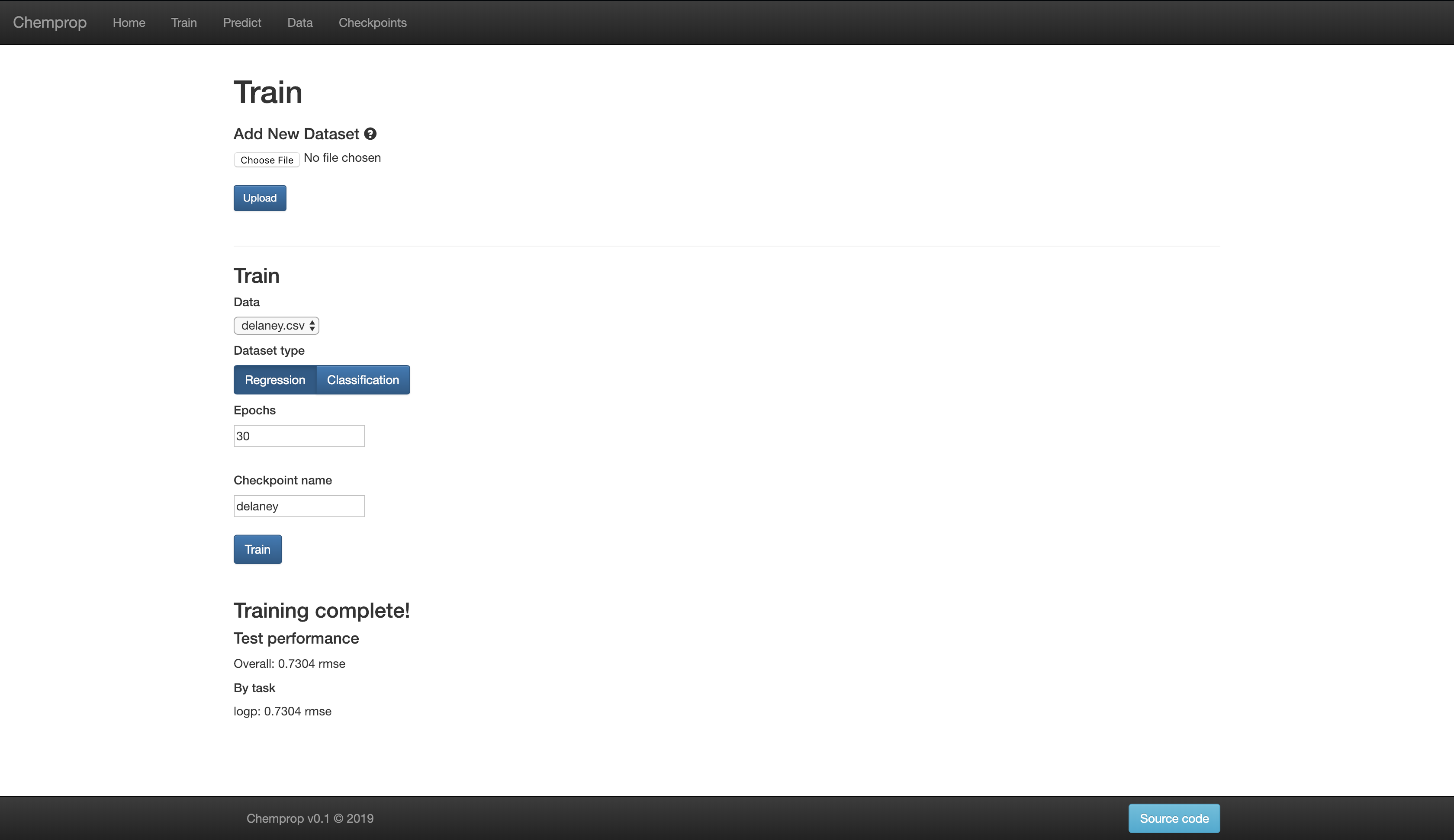
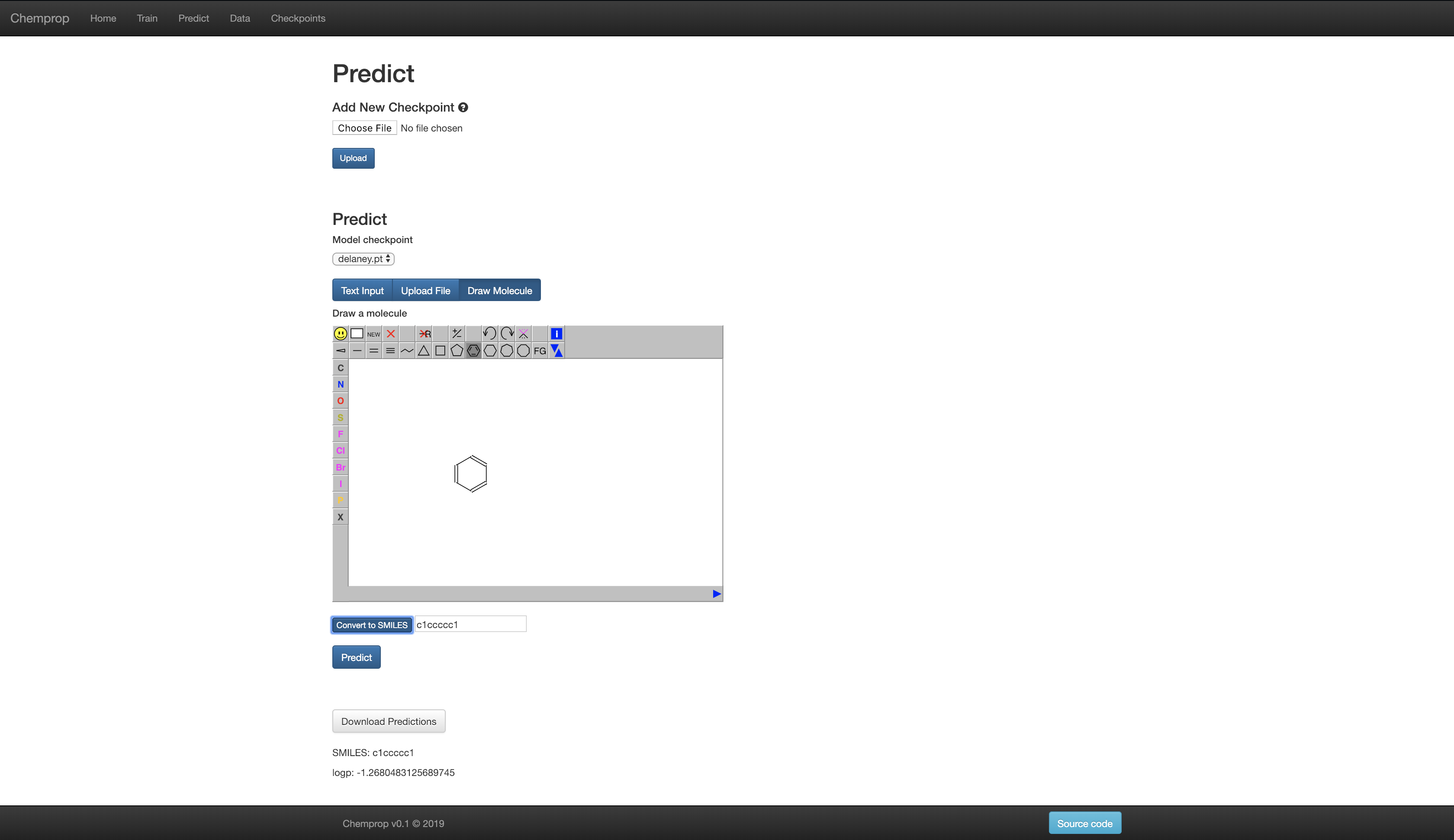
Web Interface
For those less familiar with the command line, Chemprop also includes a web interface which allows for basic training and predicting. An example of the website (in demo mode with training disabled) is available here: chemprop.csail.mit.edu.
You can start the web interface on your local machine in two ways. Flask is used for development mode while gunicorn is used for production mode.
Flask
Run chemprop_web (or optionally python web.py if installed from source) and then navigate to localhost:5000 in a web browser.
Gunicorn
Gunicorn is only available for a UNIX environment, meaning it will not work on Windows. It is not installed by default with the rest of Chemprop, so first run:
pip install gunicorn
Next, navigate to chemprop/web and run gunicorn --bind {host}:{port} 'wsgi:build_app()'. This will start the site in production mode.
- To run this server in the background, add the
--daemonflag. - Arguments including
init_dbanddemocan be passed with this pattern:'wsgi:build_app(init_db=True, demo=True)' - Gunicorn documentation can be found here.
Data
In order to train a model, you must provide training data containing molecules (as SMILES strings) and known target values. Targets can either be real numbers, if performing regression, or binary (i.e. 0s and 1s), if performing classification. Target values which are unknown can be left as blanks.
Our model can either train on a single target ("single tasking") or on multiple targets simultaneously ("multi-tasking").
The data file must be be a CSV file with a header row. For example:
smiles,NR-AR,NR-AR-LBD,NR-AhR,NR-Aromatase,NR-ER,NR-ER-LBD,NR-PPAR-gamma,SR-ARE,SR-ATAD5,SR-HSE,SR-MMP,SR-p53
CCOc1ccc2nc(S(N)(=O)=O)sc2c1,0,0,1,,,0,0,1,0,0,0,0
CCN1C(=O)NC(c2ccccc2)C1=O,0,0,0,0,0,0,0,,0,,0,0
...
By default, it is assumed that the SMILES are in the first column and the targets are in the remaining columns. However, the specific columns containing the SMILES and targets can be specified using the --smiles_column <column> and --target_columns <column_1> <column_2> ... flags, respectively.
Datasets from MoleculeNet and a 450K subset of ChEMBL from http://www.bioinf.jku.at/research/lsc/index.html have been preprocessed and are available in data.tar.gz. To uncompress them, run tar xvzf data.tar.gz.
Training
To train a model, run:
chemprop_train --data_path <path> --dataset_type <type> --save_dir <dir>
where <path> is the path to a CSV file containing a dataset, <type> is either "classification" or "regression" depending on the type of the dataset, and <dir> is the directory where model checkpoints will be saved.
For example:
chemprop_train --data_path data/tox21.csv --dataset_type classification --save_dir tox21_checkpoints
A full list of available command-line arguments can be found in chemprop/args.py.
If installed from source, chemprop_train can be replaced with python train.py.
Notes:
- The default metric for classification is AUC and the default metric for regression is RMSE. Other metrics may be specified with
--metric <metric>. --save_dirmay be left out if you don't want to save model checkpoints.--quietcan be added to reduce the amount of debugging information printed to the console. Both a quiet and verbose version of the logs are saved in thesave_dir.
Train/Validation/Test Splits
Our code supports several methods of splitting data into train, validation, and test sets.
Random: By default, the data will be split randomly into train, validation, and test sets.
Scaffold: Alternatively, the data can be split by molecular scaffold so that the same scaffold never appears in more than one split. This can be specified by adding --split_type scaffold_balanced.
Separate val/test: If you have separate data files you would like to use as the validation or test set, you can specify them with --separate_val_path <val_path> and/or --separate_test_path <test_path>.
Note: By default, both random and scaffold split the data into 80% train, 10% validation, and 10% test. This can be changed with --split_sizes <train_frac> <val_frac> <test_frac>. For example, the default setting is --split_sizes 0.8 0.1 0.1. Both also involve a random component and can be seeded with --seed <seed>. The default setting is --seed 0.
Cross validation
k-fold cross-validation can be run by specifying --num_folds <k>. The default is --num_folds 1.
Ensembling
To train an ensemble, specify the number of models in the ensemble with --ensemble_size <n>. The default is --ensemble_size 1.
Hyperparameter Optimization
Although the default message passing architecture works quite well on a variety of datasets, optimizing the hyperparameters for a particular dataset often leads to marked improvement in predictive performance. We have automated hyperparameter optimization via Bayesian optimization (using the hyperopt package), which will find the optimal hidden size, depth, dropout, and number of feed-forward layers for our model. Optimization can be run as follows:
chemprop_hyperopt --data_path <data_path> --dataset_type <type> --num_iters <n> --config_save_path <config_path>
where <n> is the number of hyperparameter settings to try and <config_path> is the path to a .json file where the optimal hyperparameters will be saved.
If installed from source, chemprop_hyperopt can be replaced with python hyperparameter_optimization.py.
Once hyperparameter optimization is complete, the optimal hyperparameters can be applied during training by specifying the config path as follows:
chemprop_train --data_path <data_path> --dataset_type <type> --config_path <config_path>
Note that the hyperparameter optimization script sees all the data given to it. The intended use is to run the hyperparameter optimization script on a dataset with the eventual test set held out. If you need to optimize hyperparameters separately for several different cross validation splits, you should e.g. set up a bash script to run hyperparameter_optimization.py separately on each split's training and validation data with test held out.
Additional Features
While the model works very well on its own, especially after hyperparameter optimization, we have seen that adding computed molecule-level features can further improve performance on certain datasets. Features can be added to the model using the --features_generator <generator> flag.
RDKit 2D Features
As a starting point, we recommend using pre-normalized RDKit features by using the --features_generator rdkit_2d_normalized --no_features_scaling flags. In general, we recommend NOT using the --no_features_scaling flag (i.e. allow the code to automatically perform feature scaling), but in the case of rdkit_2d_normalized, those features have been pre-normalized and don't require further scaling.
The full list of available features for --features_generator is as follows.
morgan is binary Morgan fingerprints, radius 2 and 2048 bits.
morgan_count is count-based Morgan, radius 2 and 2048 bits.
rdkit_2d is an unnormalized version of 200 assorted rdkit descriptors. Full list can be found at the bottom of our paper: https://arxiv.org/pdf/1904.01561.pdf
rdkit_2d_normalized is the CDF-normalized version of the 200 rdkit descriptors.
Custom Features
If you install from source, you can modify the code to load custom features as follows:
- Generate features: If you want to generate features in code, you can write a custom features generator function in
chemprop/features/features_generators.py. Scroll down to the bottom of that file to see a features generator code template. - Load features: If you have features saved as a numpy
.npyfile or as a.csvfile, you can load the features by using--features_path /path/to/features. Note that the features must be in the same order as the SMILES strings in your data file. Also note that.csvfiles must have a header row and the features should be comma-separated with one line per molecule.
Predicting
To load a trained model and make predictions, run predict.py and specify:
--test_path <path>Path to the data to predict on.- A checkpoint by using either:
--checkpoint_dir <dir>Directory where the model checkpoint(s) are saved (i.e.--save_dirduring training). This will walk the directory, load all.ptfiles it finds, and treat the models as an ensemble.--checkpoint_path <path>Path to a model checkpoint file (.ptfile).
--preds_pathPath where a CSV file containing the predictions will be saved.
For example:
chemprop_predict --test_path data/tox21.csv --checkpoint_dir tox21_checkpoints --preds_path tox21_preds.csv
or
chemprop_predict --test_path data/tox21.csv --checkpoint_path tox21_checkpoints/fold_0/model_0/model.pt --preds_path tox21_preds.csv
If installed from source, chemprop_predict can be replaced with python predict.py.
Interpreting
It is often helpful to provide explanation of model prediction (i.e., this molecule is toxic because of this substructure). Given a trained model, you can interpret the model prediction using the following command:
chemprop_interpret --data_path data/tox21.csv --checkpoint_dir tox21_checkpoints/fold_0/ --property_id 1
If installed from source, chemprop_interpret can be replaced with python interpret.py.
The output will be like the following:
- The first column is a molecule and second column is its predicted property (in this case NR-AR toxicity).
- The third column is the smallest substructure that made this molecule classified as toxic (which we call rationale).
- The fourth column is the predicted toxicity of that substructure.
As shown in the first row, when a molecule is predicted to be non-toxic, we will not provide any rationale for its prediction.
| smiles | NR-AR | rationale | rationale_score |
|---|---|---|---|
| O=[N+]([O-])c1cc(C(F)(F)F)cc([N+](=O)[O-])c1Cl | 0.014 | ||
| CC1(C)O[C@@H]2C[C@H]3[C@@H]4C[C@H](F)C5=CC(=O)C=C[C@]5(C)[C@H]4[C@@H](O)C[C@]3(C)[C@]2(C(=O)CO)O1 | 0.896 | C[C@]12C=CC(=O)C=C1[CH2:1]C[CH2:1][CH2:1]2 | 0.769 |
| C[C@]12CC[C@H]3[C@@H](CC[C@@]45O[C@@H]4C(O)=C(C#N)C[C@]35C)[C@@H]1CC[C@@H]2O | 0.941 | C[C@]12C[CH:1]=[CH:1][C@H]3O[C@]31CC[C@@H]1[C@@H]2CC[C:1][CH2:1]1 | 0.808 |
| C[C@]12C[C@H](O)[C@H]3[C@@H](CCC4=CC(=O)CC[C@@]43C)[C@@H]1CC[C@]2(O)C(=O)COP(=O)([O-])[O-] | 0.957 | C1C[CH2:1][C:1][C@@H]2[C@@H]1[C@@H]1CC[C:1][C:1]1C[CH2:1]2 | 0.532 |
Chemprop's interpretation script explains model prediction one property at a time. --property_id 1 tells the script to provide explanation for the first property in the dataset (which is NR-AR). In a multi-task training setting, you will need to change --property_id to provide explanation for each property in the dataset.
For computational efficiency, we currently restricted the rationale to have maximum 20 atoms and minimum 8 atoms. You can adjust these constraints through --max_atoms and --min_atoms argument.
TensorBoard
During training, TensorBoard logs are automatically saved to the same directory as the model checkpoints. To view TensorBoard logs, run tensorboard --logdir=<dir> where <dir> is the path to the checkpoint directory. Then navigate to http://localhost:6006.
Results
We compared our model against MolNet by Wu et al. on all of the MolNet datasets for which we could reproduce their splits (all but Bace, Toxcast, and qm7). When there was only one fold provided (scaffold split for BBBP and HIV), we ran our model multiple times and reported average performance. In each case we optimize hyperparameters on separate folds, use rdkit_2d_normalized features when useful, and compare to the best-performing model in MolNet as reported by Wu et al. We did not ensemble our model in these results.
Results on regression datasets (lower is better)
| Dataset | Size | Metric | Ours | MolNet Best Model |
|---|---|---|---|---|
| QM8 | 21,786 | MAE | 0.011 ± 0.000 | 0.0143 ± 0.0011 |
| QM9 | 133,885 | MAE | 2.666 ± 0.006 | 2.4 ± 1.1 |
| ESOL | 1,128 | RMSE | 0.555 ± 0.047 | 0.58 ± 0.03 |
| FreeSolv | 642 | RMSE | 1.075 ± 0.054 | 1.15 ± 0.12 |
| Lipophilicity | 4,200 | RMSE | 0.555 ± 0.023 | 0.655 ± 0.036 |
| PDBbind (full) | 9,880 | RMSE | 1.391 ± 0.012 | 1.25 ± 0 |
| PDBbind (core) | 168 | RMSE | 2.173 ± 0.090 | 1.92 ± 0.07 |
| PDBbind (refined) | 3,040 | RMSE | 1.486 ± 0.026 | 1.38 ± 0 |
Results on classification datasets (higher is better)
| Dataset | Size | Metric | Ours | MolNet Best Model |
|---|---|---|---|---|
| PCBA | 437,928 | PRC-AUC | 0.335 ± 0.001 | 0.136 ± 0.004 |
| MUV | 93,087 | PRC-AUC | 0.041 ± 0.007 | 0.184 ± 0.02 |
| HIV | 41,127 | ROC-AUC | 0.776 ± 0.007 | 0.792 ± 0 |
| BBBP | 2,039 | ROC-AUC | 0.737 ± 0.001 | 0.729 ± 0 |
| Tox21 | 7,831 | ROC-AUC | 0.851 ± 0.002 | 0.829 ± 0.006 |
| SIDER | 1,427 | ROC-AUC | 0.676 ± 0.014 | 0.648 ± 0.009 |
| ClinTox | 1,478 | ROC-AUC | 0.864 ± 0.017 | 0.832 ± 0.037 |
Lastly, you can find the code to our original repo at https://github.com/wengong-jin/chemprop and for the Mayr et al. baseline at https://github.com/yangkevin2/lsc_experiments .
Project details
Release history Release notifications | RSS feed


Download files
Download the file for your platform. If you're not sure which to choose, learn more about installing packages.
Source Distribution
File details
Details for the file chemprop-1.0.1.tar.gz.
File metadata
- Download URL: chemprop-1.0.1.tar.gz
- Upload date:
- Size: 66.8 kB
- Tags: Source
- Uploaded using Trusted Publishing? No
- Uploaded via: twine/3.2.0 pkginfo/1.5.0.1 requests/2.24.0 setuptools/49.1.0.post20200704 requests-toolbelt/0.9.1 tqdm/4.47.0 CPython/3.7.6
File hashes
| Algorithm | Hash digest | |
|---|---|---|
| SHA256 |
70d0a38878d851f1d01c8f095802727ed85f84152da0a33d7d2b6f295ee561ee
|
|
| MD5 |
41121557eb0ab9ebcabaffcf7ec34414
|
|
| BLAKE2b-256 |
382af6fc398584b7d35b4e677815f28bc74725cce342a9d428bcd6525f59f315
|


