
chromabench
A minimal validation for chromatic topological data analysis.
If you have a method that is meant to see the shape and colour distribution of a point cloud at the same time, chromabench is the first, simplest check that it actually does.
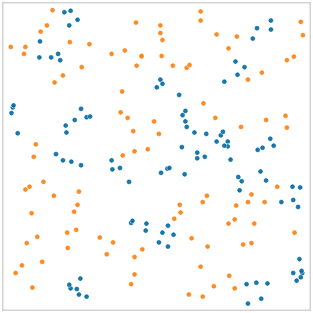
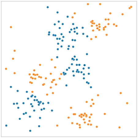
It is a 2x2 family of two-colour point clouds: two spatial distributions, uniform or cluster, and each with colours either mixed or separated.
Because the mixed and separated versions of a layout reuse the same points, only the colour distribution tells them apart.
Install
pip install chromabench
At a glance
chromabench provides two functionalities: load_dataset(), which builds the benchmark point clouds, and evaluate(method, dataset), which scores a method against the colour-blind PH baseline.
A method is any object with a fit(samples, y) and a predict(samples). Here samples is a list of point clouds -- each a dict with two keys, "coords" (an (n, 2) array of point positions) and "colours" (an (n,) array of 0/1 labels) -- and y is the array of class indices.
The evaluation score is balanced accuracy under 10-fold cross-validation (chance = 0.25).
from chromabench import evaluate, load_dataset

ds = load_dataset()
print(evaluate(MyChromaticMethod(), ds)["score"])     # your method
The data
Each sample is a two-colour point cloud in the unit square.
The four classes factor as spatial distribution x colour distribution (class name = <spatial>_<colour>):
Within each row the mixed and separated point clouds are sampled from the same spatial distribution and only the colour distribution changes.
- spatial (
uniform/cluster): how the points are distributed in space. - colour (
mixed/separated): how the two colours are distributed over those points, with the spatial layout held fixed.
In every class the two colours are balanced (100 points each). mixed assigns those colours uniformly at random, so colour carries no spatial signal. separated assigns colours such that colours are clustered in space. See the details below for more information.
| mixed | separated | |
|---|---|---|
| uniform | 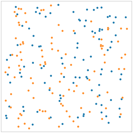 |
 |
| cluster | 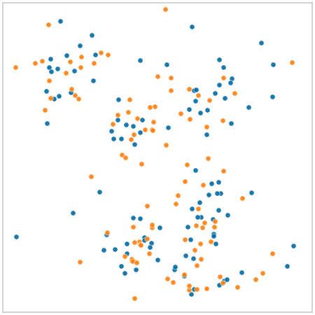 |
 |
Details
We first sample points from the corresponding spatial distribution and then colour them using the specified colouring scheme.
Each realization has n_A = n_B = 100.
Spatial layout.
A uniform cloud is n_A + n_B = 200 i.i.d. uniform points on [0,1]^2.
A cluster cloud draws K = 6 well-spaced centres and splits the points into background and clustered counts
$$n_\text{bg} = \operatorname{round}!\big(f_\text{bg},(n_A + n_B)\big), \qquad n_\text{cluster} = n_A + n_B - n_\text{bg},$$
with background fraction f_bg = 0.15; background points are uniform and clustered points are Gaussian (σ = 0.065) around the centres, clipped to [0,1]^2.
Colouring.
mixed colours exactly n_A = 100 points chosen uniformly at random as A and the rest as B.
separated depends on the layout:
uniform_separated: complete-linkage hierarchical clustering of the points; small clusters are ordered by increasing merge height, points within a cluster by distance to its centroid, and the first 100 in that order are coloured A.cluster_separated: theKcentres are split evenly between the colours; clustered points inherit their centre's colour and background points take their nearest centre's colour, with the counts adjusted if necessary to keep the 100/100 balance exact.
Data generation
load_dataset() builds the whole benchmark and hands it back as a single Dataset.
With the defaults it generates 400 point clouds (four classes, 100 samples each), each a set of 200 points in the unit square carrying a 0/1 colour label, plus a class index y for every sample: 0 = uniform_mixed, 1 = uniform_separated, 2 = cluster_mixed, 3 = cluster_separated.
from chromabench import load_dataset

ds = load_dataset()          # 4 classes x 100 samples, seed 42
ds.samples                   # list of {"coords": (n, 2), "colours": (n,)}
ds.y                         # class index per sample
ds.class_names               # ("uniform_mixed", "uniform_separated", ...)
load_dataset() accepts n_per_class, seed, and params if you want to vary the size or regenerate; the defaults reproduce the benchmark.
To draw a single point cloud, e.g. to use the generator as a stand-alone data model, call simulate directly:
from chromabench import simulate
import numpy as np

sample = simulate("cluster_separated", rng=np.random.default_rng(0), params=None)
sample["coords"], sample["colours"]
Evaluation
evaluate(method, dataset) scores a method with stratified 10-fold cross-validation: in each fold the method is fit on the training point clouds and predicts the held-out ones, and the pooled out-of-fold predictions are scored. The metric is balanced accuracy (macro-averaged recall; chance = 0.25 for the four balanced classes).
from chromabench import evaluate, load_dataset

result = evaluate(MyChromaticMethod(), load_dataset())
result["score"]      # {"balanced_accuracy": ...}
See examples/validate_method.py.
The baseline: Ordinary Persistent Homology
Persistent homology (PH) of the pooled points (colours discarded) depends only on the spatial layout.
The mixed and separated members of a class share the same point positions, so they are topologically identical to PH.
A multiclass logistic regression on the PH features (persistence images of the pooled points) therefore recovers uniform vs cluster, but has to guess between mixed and separated.
from chromabench import load_dataset, run_baseline

ds = load_dataset()
print(run_baseline(ds)["score"])             # ordinary PH (colour-blind)
The baseline is itself a Method: PHBaseline implements the same fit/predict interface a submission does -- run_baseline is just evaluate(PHBaseline()) -- so it doubles as a complete, copyable example of how to wire one up.
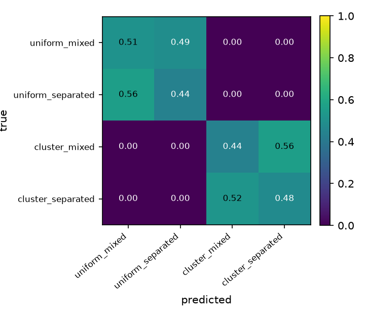
Confusion matrix of the colour-blind PH reference, aggregated over 10-fold cross-validation (rows normalised). PH never crosses spatial layouts, but splits mixed vs separated at roughly chance within each.
Citation
This is exactly what GitHub's "Cite this repository" button emits from CITATION.cff -- keep the two in sync.
@software{Bleher_chromabench_2026,
author = {Bleher, Michael},
license = {MIT},
month = jun,
title = {{chromabench}},
url = {https://github.com/subthaumic/chromabench},
version = {0.1.0},
year = {2026}
}
License
MIT.
1 maintainer

Metadata
1 maintainer
Release files for chromabench 0.1.0
For a detailed explanation of source distributions (sdists) and built distributions (wheels), please see the package formats documentation.
Source distribution (sdist)
| File | Size | Uploaded | |
|---|---|---|---|
| chromabench-0.1.0.tar.gz | 183.7 kB | Details |
Built distribution (wheel)
| File | Interpreter | ABI | Platform | Reset |
|---|---|---|---|---|
| chromabench-0.1.0-py3-none-any.whl | Python 3 | none | any | Details |
Total release size: 198.0 kB
Release files / chromabench-0.1.0.tar.gz
| Download URL | chromabench-0.1.0.tar.gz |
|---|---|
| Size | 183.7 kB |
| Tags | Source |
|
SHA-256 checksum How to use checksums |
a7666a08e9aac16410a8bef7bd896571d29a542543adf974859acd8ef93c4f9f
|
|
BLAKE2b-256 checksum How to use checksums |
decfa269ff043e2aabe0dac9e007bc9a57e2e2824b67a1aecfa6d21a718eb74c
|
| Upload date | |
|
Uploaded using Trusted Publishing? What is trusted publishing? |
No |
| Uploaded via |
twine/7.0.0 CPython/3.13.14
|
Release files / chromabench-0.1.0-py3-none-any.whl
| Download URL | chromabench-0.1.0-py3-none-any.whl |
|---|---|
| Size | 14.3 kB |
| Tags | Python 3 |
|
SHA-256 checksum How to use checksums |
6069735d9ba777ecc51e53435a7f19cdef9be1df90ecb388e3d9b0f406246b06
|
|
BLAKE2b-256 checksum How to use checksums |
2252abc829ee9714f253939fabc7567c5cc9ad6f2174c8685546d01d76b37fb7
|
| Upload date | |
|
Uploaded using Trusted Publishing? What is trusted publishing? |
No |
| Uploaded via |
twine/7.0.0 CPython/3.13.14
|













