No project description provided

Project description
ClaSPy: A Python package for time series segmentation


Time series segmentation (TSS) tries to partition a time series (TS) into semantically meaningful segments. It's an important unsupervised learning task applied to large, real-world sensor signals for human inspection, change point detection or as preprocessing for classification and anomaly detection. This python library is the official implementation of the accurate and domain-agnostic TSS algorithm ClaSP.
Installation
You can install ClaSPy with PyPi:
python -m pip install claspy
Usage: univariate time series
Let's first import the ClaSP algorithm and univariate TS data from the "Time Series Segmentation Benchmark" (TSSB) to demonstrate its utility.
>>> from claspy.segmentation import BinaryClaSPSegmentation
>>> from claspy.data_loader import load_tssb_dataset
As an example, we choose the Cricket data set that contains motions of different umpire signals captured as wrist acceleration. ClaSP should automatically detect semantic changes between signals and deduce their segmentation. It is parameter-free, so we just need to pass the time series as a numpy array.
>>> dataset, window_size, true_cps, labels, time_series = load_tssb_dataset(names=("CricketX",)).iloc[0,:]
>>> clasp = BinaryClaSPSegmentation()
>>> clasp.fit_predict(time_series)
[ 712 1281 1933 2581]
ClaSP is fully interpretable to human inspection. It creates a score profile (between 0 and 1) that estimates the probability of a "change point" in a TS, where one segment transitions into another. We visualize the segmentation and compare it to the pre-defined human annotation.
>>> clasp.plot(gt_cps=true_cps, heading="Segmentation of different umpire cricket signals", ts_name="ACC", file_path="segmentation_example.png")
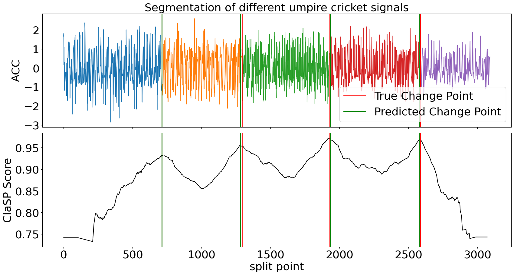
ClaSP accurately detects the number and location of changes in the motion sequence (compare green vs red lines) that infer its segmentation (the different-coloured subsequences). It is carefully designed to do this fully autonomously. However, if you have domain-specific knowledge, you can utilize it to guide and improve the segmentation. See its parameters for more information.
Usage: multivariate time series
Now, let's import multivariate TS data from the "Human Activity Segmentation Challenge" to show how ClaSP handles it.
>>> from claspy.data_loader import load_has_dataset
In this example, we use a motion routine from a student getting on, riding, and getting of a train. The multivariate TS consists of acceleration and magnetometer readings from a smartphone. We pass the time series as a 2-dimensional numpy array to ClaSP.
>>> dataset, window_size, true_cps, labels, time_series = load_has_dataset().iloc[107, :]
>>> clasp = BinaryClaSPSegmentation()
>>> clasp.fit_predict(time_series)
[ 781 8212 9287 14468]
We visualize the segmentation and compare it to the ground truth annotation.
>>> clasp.plot(gt_cps=true_cps, heading=f"Segmentation of activity routine: {', '.join(labels)}", ts_name="ACC", font_size=18, file_path="multivariate_segmentation_example.png")
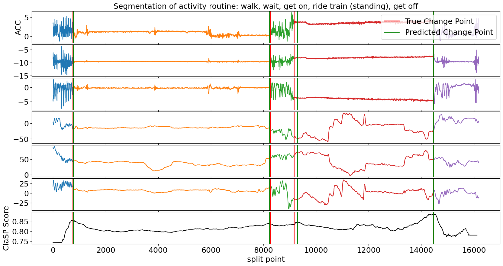
Also in the multivariate case, ClaSP correctly determines the number und location of activities in the routine. It is built to extract information from all TS channels to guide the segmentation. To ensure high performance, only provide necessary TS dimensions to ClaSP.
Usage: streaming time series
We also provide a streaming implementation of ClaSP that can segment ongoing time series streams or very large data archives in real-time (few thousand observations per second).
>>> from claspy.streaming.segmentation import StreamingClaSPSegmentation
In our example, we simulate an ongoing ECG time series stream and use ClaSP to detect the transition between normal heartbeats and a myocardial infarction as soon as possible. We use a sliding window of 1k data points and update ClaSP with every data point.
>>> dataset, window_size, true_cps, labels, time_series = load_tssb_dataset(names=("ECG200",)).iloc[0, :]
>>> clasp = StreamingClaSPSegmentation(n_timepoints=1000)

>>> for idx, value in enumerate(time_series):
>>>     clasp.update(value)
>>>     if idx >= clasp.n_warmup and clasp.predict() != 0:
>>>         break
For the first 1k data points, ClaSP "warms up", which means that it learns internal parameters from the data. Thereafter, we can query its predict method to find the last change point, e.g. to alert the user in real-time. In this example we wait for the first change point to occur and then inspect the sliding window.
>>> clasp.plot(heading="Detection of myocardial infarction in ECG stream", stream_name="ECG", file_path=f"streaming_segmentation_example.png")
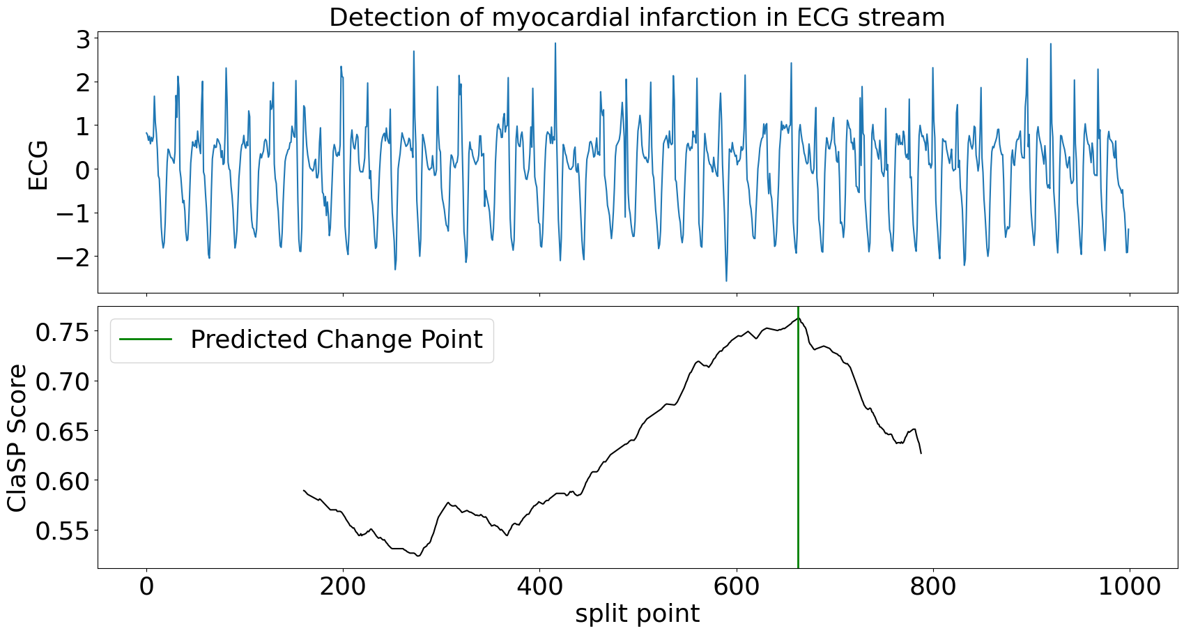
ClaSP needs circa 300 data points to accurately detect the change in heart beats. After the alert, it can be continued to be updated to detect more changes in the future. ClaSP is designed to automatically expel old data from its sliding window, efficiently use memory and run indefinitely. See this tutorial for more information.
Extension: state detection
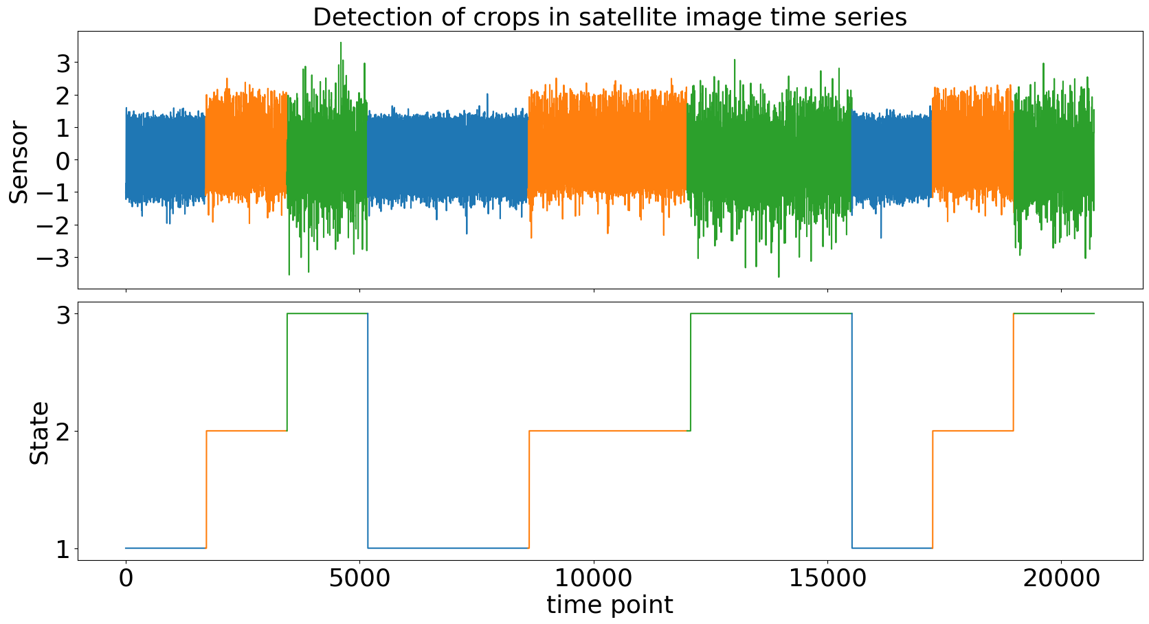
We extend TSS with state detection to infer latent system states from TS data and to recover their transition structure. This is particularly useful when segments correspond to recurring regimes (e.g., crop types in satellite image TS), where both the ordering and repetition of states matter.
We demonstrate state detection with the CLaP algorithm on the Crop dataset from the TSSB, where a satellite image TS captures different crops (one per colour). The goal is to automatically identify the underlying states and their transitions.
>>> from claspy.state_detection import AgglomerativeCLaPDetection
Similar to ClaSP, CLaP is parameter-free and directly returns a state sequence, assigning a discrete state label to each time point. These states label segments in the TS (e.g., different crops).
>>> dataset, window_size, true_cps, labels, time_series = load_tssb_dataset(names=("Crop",)).iloc[0, :]
>>> clap = AgglomerativeCLaPDetection()
>>> state_seq = clap.fit_predict(time_series)
We can visualize the detected state sequence and compare it to the ground truth.
>>> clap.plot(gt_states=labels, heading="Detection of crops in satellite image time series", ts_name="Sensor", file_path=f"state_detection_example.png")
Beyond labeling, CLaP can recover the process structure underlying the TS by abstracting states and transitions:
>>> states, transitions = clap.predict(sparse=True)
{1, 2, 3}
{(1, 2), (2, 3), (3, 1)}
Here, each state corresponds to a crop type, and transitions describe how the system evolves over time. We can visualize this as a state transition graph:
>>> clap.plot(heading="Process of captured crops", file_path=f"process_discovery_example.png", sparse=True)
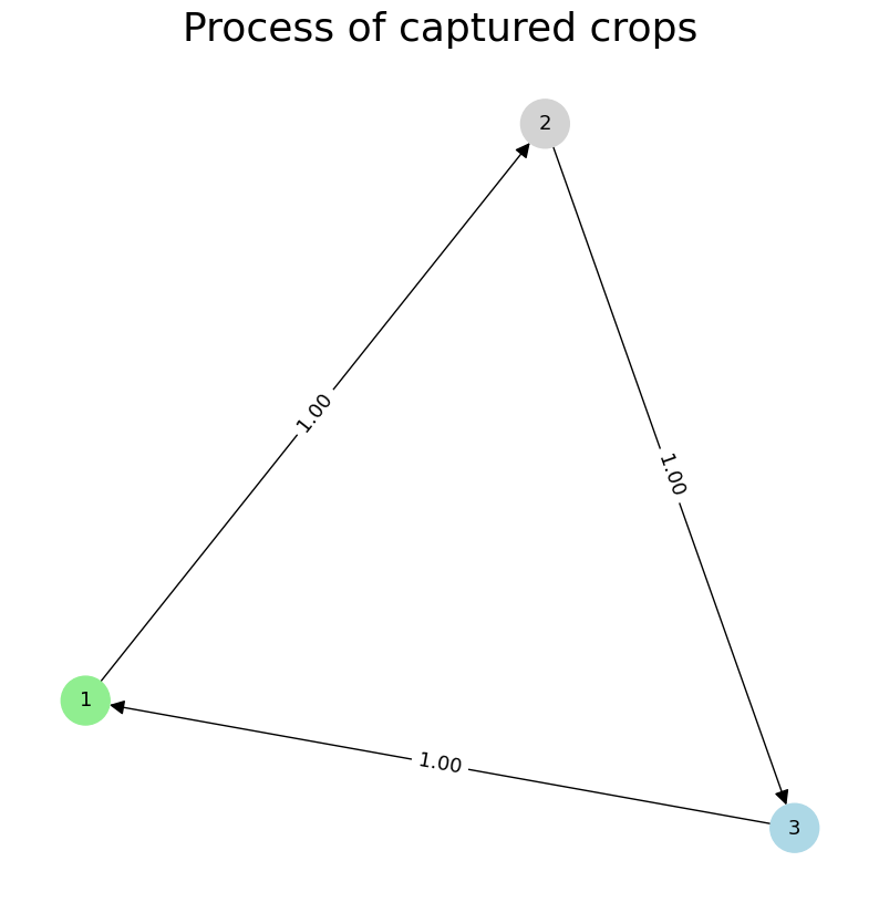
This representation abstracts the TS into a compact process model, where nodes represent states and edges indicate observed transitions. It enables downstream analysis such as anomaly detection, or classification on state-labeled sequences.
The state detection workflow complements segmentation by not only identifying boundaries but also assigning consistent semantic labels across recurring segments, allowing a higher-level understanding of temporal dynamics.
Examples
Checkout the following Jupyter notebooks that show applications of the ClaSPy package:
- ClaSP evaluation on the "Time Series Segmentation Benchmark" (TSSB)
- ClaSP results for the "Human Activity Segmentation Challenge"
- Hyper-parameter Tuning and Configuration of ClaSP
- Window Size Selection for Unsupervised Time Series Analytics
- Segmentation of Streaming Time Series and Large Data Archives
Citation
The ClaSPy package is actively maintained, updated and intended for application. If you use ClaSP/ClaSS/CLaP in your scientific publication, we would appreciate the corresponding citation:
@article{Ermshaus2023ClaSP,
  title={ClaSP: parameter-free time series segmentation},
  author={Arik Ermshaus and Patrick Sch{\"a}fer and Ulf Leser},
  journal={Data Mining and Knowledge Discovery},
  year={2023},
  volume={37},
  pages={1262-1300},
}

@article{Ermshaus2024ClaSS,
  title={Raising the ClaSS of Streaming Time Series Segmentation},
  author={Arik Ermshaus and Patrick Sch{\"a}fer and Ulf Leser},
  journal={Proceedings of the VLDB Endowment},
  volume={17},
  number={8},
  pages={1953-1966},
  year={2024},
  publisher={VLDB Endowment}
}

@article{Ermshaus2025CLaP,
  title={CLaP - State Detection from Time Series},
  author={Arik Ermshaus and Patrick Sch{\"a}fer and Ulf Leser},
  journal={Proceedings of the VLDB Endowment},
  volume={19},
  number={1},
  pages={70-83},
  year={2025},
  publisher={VLDB Endowment}
}
Todos
Here are some of the things we would like to add to ClaSPy in the future:
- Future research related to ClaSP
- Example and application Jupyter notebooks
- More documentation and tests
If you want to contribute, report bugs, or need help applying ClaSP for your application, feel free to reach out.
Release history Release notifications | RSS feed


Download files
Download the file for your platform. If you're not sure which to choose, learn more about installing packages.
Source Distribution
Built Distribution
Filter files by name, interpreter, ABI, and platform.
If you're not sure about the file name format, learn more about wheel file names.
Copy a direct link to the current filters
File details
Details for the file claspy-0.2.8.tar.gz.
File metadata
- Download URL: claspy-0.2.8.tar.gz
- Upload date:
- Size: 57.2 kB
- Tags: Source
- Uploaded using Trusted Publishing? No
- Uploaded via: twine/6.1.0 CPython/3.9.18
File hashes
| Algorithm | Hash digest | |
|---|---|---|
| SHA256 |
b98ee65ac11845df89af9f68d31caa9a101cd77392412e1689a0292384815684
|
|
| MD5 |
105ec9f7b34d67621cd35720cc85f0b4
|
|
| BLAKE2b-256 |
ee47f46789b4ad2457eb7349e37120c6c34478b5b9b596f032884814d684588e
|
File details
Details for the file claspy-0.2.8-py3-none-any.whl.
File metadata
- Download URL: claspy-0.2.8-py3-none-any.whl
- Upload date:
- Size: 65.4 kB
- Tags: Python 3
- Uploaded using Trusted Publishing? No
- Uploaded via: twine/6.1.0 CPython/3.9.18
File hashes
| Algorithm | Hash digest | |
|---|---|---|
| SHA256 |
e761f76216f1cc04e17e48f24d38247940694d0b9c050b89f6b1a5b572555016
|
|
| MD5 |
2a9fd73fe8a0af4872fdf2ab632f0085
|
|
| BLAKE2b-256 |
91bccd211e4a436f0d4f6338d183829b38899a9ae2b24340a5a77250012b205f
|


