
Combinatorial h+/e- Sample Investigation using Voltaic Measurements

Project description
COHESIVM: Combinatorial h+/e- Sample Investigation using Voltaic Measurements
Introduction
The COHESIVM Python package provides a generalized framework for conducting combinatorial voltaic measurements in
scientific research and development. The modular architecture enables researchers to adapt it to diverse experimental
setups by extending its components to support custom configurations. These components are cohesively put together in an
Experiment class which runs compatibility checks, manages data storage, and
executes the measurements.
Key Features:
- Modular Design: COHESIVM adopts a module-oriented approach where components such as measurement devices
(
Device), contacting interfaces (Interface), and measurement routines (Measurement) are abstracted into interchangeable units. This modular architecture enhances flexibility in experimental setups and makes it easy to add new component implementations. The tutorials in the documentation provide an extensive description of implementing custom components. - Combinatorial Flexibility: By abstracting the class for the contacting interface, COHESIVM enables diverse
configurations for sample investigation. The MA8X8 measurement array, as implemented in the current core
version, is only one example for an electrode contact array. Researchers can add custom implementations of the
Interfaceclass to support other configurations or, for example, robotic contacting systems. - Data Handling: Collected data is stored in a structured HDF5 database
format using the
Databaseclass, ensuring efficient data management and accessibility.Metadatais collected based on the DCMI standard which is extended by COHESIVM-specific metadata terms. - Analysis and GUIs: Alongside the measurement routines, analysis functions and plots can be implemented, extending
the
Analysisbase class. Together with the graphical user interface (also available for conducting experiments and reviewing the database contents), initial screening of the data is facilitated.
Table of Contents
Getting Started
Dependencies
The current core version of COHESIVM is tested for Python 3.9–3.12 and requires the following dependencies:
- h5py (~=3.8)
- numpy (~=1.21)
- matplotlib (~=3.7)
- tqdm (~=4.65)
Apart from the core package, extras
exist for modules with additional dependencies (check the pyproject.toml for a complete listing):
| Extra | Module | Dependency |
|---|---|---|
| gui | cohesivm.gui | bqplot~=0.12 |
| ma8x8 | cohesivm.interfaces.ma8x8 | pyserial~=3.5 |
| ossila | cohesivm.devices.ossila | xtralien~=2.10 |
| agilent | cohesivm.devices.agilent | pyvisa~=1.13 |
| full | – | all from above |
Installation
Using pip
To install the core COHESIVM package from the Python Package Index (PyPI), simply run:
pip install cohesivm
This command will download and install the latest stable version of COHESIVM and its core dependencies.
[!IMPORTANT]
If you want to use the GUIs inside your Jupyter environment, make sure to specify the
guiextra:pip install cohesivm[gui]
Cloning from GitHub
If you want to install the development version of the package from the GitHub repository, follow these steps:
- Clone the repository to your local machine:
git clone https://github.com/mxwalbert/cohesivm.git - Navigate into the cloned directory:
cd cohesivm - Install the package and its dependencies:
pip install .[dev]
Configuration
A config.ini file should be placed in the root of your project to configure the hardware ports/addresses of the
contact interfaces and measurement devices. Some DCMI metadata terms also need to be defined there. COHESIVM implements
a config parser which allows to access these values, e.g.:
>>> import cohesivm
>>> cohesivm.config.get_option('DCMI', 'creator')
Dow, John
Template
A preconfigured file with the currently implemented interfaces and devices can be copied from the repository, or you can create your own from this template:
# This file is used to configure the project as well as the devices and interfaces (e.g., COM ports, addresses, ...).

# METADATA ------------------------------------------------------------------------------------------------------------

[DCMI]
# The following options correspond to the terms defined by the Dublin Core Metadata Initiative.
# See https://purl.org/dc/terms/ for detailed descriptions.
publisher = "Your Company Ltd."
creator = "Dow, John"
rights = <https://link.to/licence>
subject = "modular design"; "combinatorial flexibility"; "data handling"; "analysis and gui"

# ---------------------------------------------------------------------------------------------------------------------


# INTERFACES ----------------------------------------------------------------------------------------------------------

[NAME_OF_USB_INTERFACE]
com_port = 42

# ---------------------------------------------------------------------------------------------------------------------


# DEVICES -------------------------------------------------------------------------------------------------------------

[NAME_OF_NETWORK_DEVICE]
address = localhost
port = 8888
timeout = 0.1

# ---------------------------------------------------------------------------------------------------------------------
The names of the sections (e.g., NAME_OF_USB_INTERFACE) must be unique but can be chosen freely since they are
referenced manually. The options (e.g., com_port), on the other hand, should follow the signature of the class
constructor to use them efficiently. For example, an Interface implementation
DemoInterface which requires the com_port parameter could be initialized using the configuration template
from above:
interface = DemoInterface(**config.get_section('NAME_OF_USB_INTERFACE'))
Example
In a common scenario, you probably want to configure multiple devices to use them at once. Let's consider the case
where you need two OssilaX200 devices which are both connected via USB. Then, in the
DEVICES part of the configuration, you would define two distinctive sections and set the required address
option:
# DEVICES -------------------------------------------------------------------------------------------------------------

[OssilaX200_1]
address = COM4

[OssilaX200_2]
address = COM5

# ---------------------------------------------------------------------------------------------------------------------
To initialize the devices, you could do something similar to the Basic Usage example:
from cohesivm import config
from cohesivm.devices.ossila import OssilaX200
smu1 = OssilaX200.VoltageSMUChannel()
device1 = OssilaX200.OssilaX200(channels=[smu1], **config.get_section('OssilaX200_1'))
smu2 = OssilaX200.VoltageSMUChannel()
device2 = OssilaX200.OssilaX200(channels=[smu2], **config.get_section('OssilaX200_2'))
Basic Usage
[!IMPORTANT] If you only installed the core package, the following example will raise import errors from missing dependencies. To use the
Agilent4156C,MA8X8, andOssilaX200classes, you need to install theagilent,ma8x8, andossilaextras, respectively. To add all dependencies at once, install thefullextra with this command:pip install cohesivm[full]
With working implementations of the main components (Device,
Interface, Measurement), setting up and running an
experiment only takes a few lines of code:
from cohesivm import config
from cohesivm.database import Database, Dimensions
from cohesivm.experiment import Experiment
from cohesivm.progressbar import ProgressBar
from cohesivm.devices.agilent import Agilent4156C
from cohesivm.interfaces import MA8X8
from cohesivm.measurements.iv import CurrentVoltageCharacteristic

# Create a new or load an existing database
db = Database('Test.h5')

# Configure the components
smu = Agilent4156C.SweepVoltageSMUChannel()
device = Agilent4156C.Agilent4156C(channels=[smu], **config.get_section('Agilent4156C'))
interface = MA8X8(com_port=config.get_option('MA8X8', 'com_port'), pixel_dimensions=Dimensions.Circle(radius=0.425))
measurement = CurrentVoltageCharacteristic(start_voltage=-2.0, end_voltage=2.0, voltage_step=0.01, illuminated=True)

# Combine the components in an experiment
experiment = Experiment(
    database=db,
    device=device,
    interface=interface,
    measurement=measurement,
    sample_id='test_sample_42',
    selected_contacts=None
)

# Optionally set up a progressbar
pbar = ProgressBar(experiment)

# Run the experiment
with pbar.show():
    experiment.quickstart()
If you want to change the measurement device to a different one, you only need to adjust the lines for the
Channel and the Device accordingly:
from cohesivm.devices.ossila import OssilaX200
smu = OssilaX200.VoltageSMUChannel()
device = OssilaX200.OssilaX200(channels=[smu], **config.get_section('OssilaX200'))
Graphical User Interfaces
If you work with Jupyter, you may use the Graphical User Interfaces (GUIs) which are implemented in the form of Jupyter Widgets.
Currently, three GUIs are available:
Experiment GUI
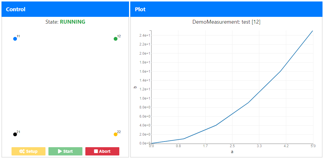
ExperimentState, followed by a
representation of the Interface and the control buttons at the bottom. The circles are
annotated with the contact_ids and the colors correspond to their current state.
On the right panel "Plot", the currently running Measurement is displayed. The plot is
automatically updated as soon as new measurement data arrives in the
data_stream of the Experiment object.
Database GUI
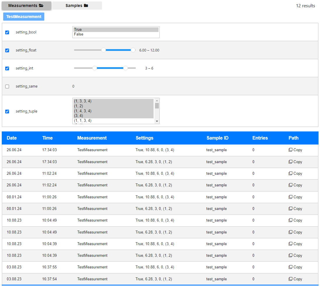
Measurement or by the
sample_name of the Experiment object. If you
choose the former one, you may additionally filter the data by means of measurement parameters. The button to the very
right of each data row enables you to copy the dataset path, to access it in the Database.
Analysis GUI
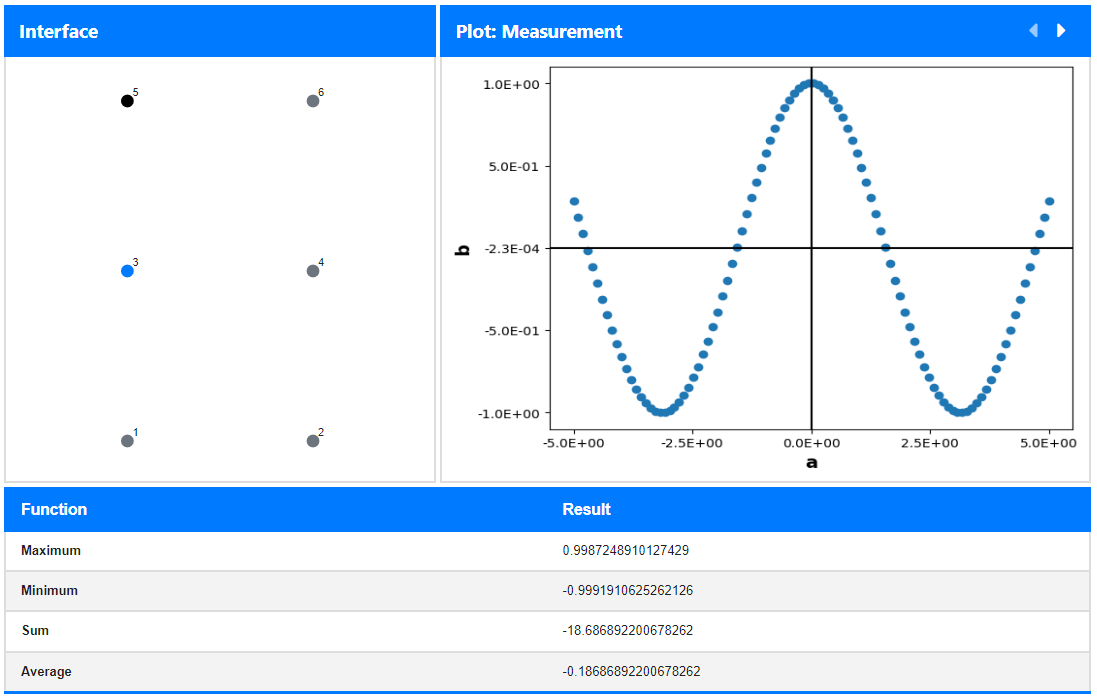
functions that are defined in the Analysis class. The
results of the functions, which are also implemented there, are shown in the table
below.
Detailed guides to work with the GUIs can be found in the documentation.
Examples
[!NOTE] For a practical example, read the Real-World Example.
Run an Experiment
Follow the Basic Usage example to set up and run an
Experiment. If you do not have all components ready yet, follow these tutorials:
To follow the other examples you may just run the code from the Basic Usage example even if you do not have access to the hardware. This will fail but create an HDF5 file and store an empty dataset entry.
Manage the Data
After you collected some data and stored it in an HDF5 file, you can use the Database class
to work with it. First, initialise the Database object and list the samples which are stored
there:
>>> from cohesivm.database import Database
>>> db = Database('Test.h5')
>>> db.get_sample_ids()
['test_sample_42']
This is exactly the sample_id which was specified when the
Experiment was configured, and it can be used to retrieve the actual
dataset path in the Database object:
>>> db.filter_by_sample_id('test_sample_42')
['/CurrentVoltageCharacteristic/55d96687ee75aa11:26464063430fe52f:a69a946e7a02e547:c8965a35118ce6fc:67a8bfb44702cfc7:8131a44cea4d4bb8/2024-07-01T10:44:59.033161-test_sample_42']
The resulting list contains the path strings for all experiments with the specified
sample_id (currently only one entry). These strings get quite long because they
contain the name of the Measurement
procedure, followed by a hashed representation of the settings dictionary,
and finally the datetime combined with the sample_id. With this
dataset path, you may retrieve some information from the
Metadata object which got created by the Experiment:
>>> dataset = db.filter_by_sample_id('test_sample_42')[0]
>>> metadata = db.load_metadata(dataset)
>>> metadata.sample_id, metadata.device, metadata.interface, metadata.measurement
('test_sample_42', 'Agilent4156C', 'MA8X8', 'CurrentVoltageCharacteristic')
Storing a new dataset is less trivial because you need a fully qualified Metadata object,
which asks for a large number of arguments. Anyway, this is usually handled by the
Experiment class because it guarantees that the specified components are compatible. For
testing, the Metadata object from above may be used to initialize a new dataset:
>>> db.initialize_dataset(metadata)
'/CurrentVoltageCharacteristic/55d96687ee75aa11:26464063430fe52f:a69a946e7a02e547:c8965a35118ce6fc:67a8bfb44702cfc7:8131a44cea4d4bb8/2024-07-01T10:46:05.910371-test_sample_42'
This yields practically the same dataset path as before, only the datetime is different. Adding data entries, on
the other hand, is fairly simple because you only need to specify the dataset and the contact_id (alongside
the data of course):
>>> db.save_data(np.array([1]), dataset)
>>> db.save_data(np.array([42]), dataset, '1')
Finally, you may load a data entry by specifying the contact_id (or a list of several) or load an entire dataset,
including the Metadata:
>>> db.load_data(dataset, '0')
[array([1])]
>>> db.load_data(dataset, ['0', '1'])
[array([1]), array([42])]
>>> db.load_dataset(dataset)
({'0': array([1]), '1': array([42])}, Metadata(CurrentVoltageCharacteristic, Agilent4156C, MA8X8))
The Database class also implements methods for filtering datasets based on
settings of the Measurement. Check out the
documentation of the filter_by_settings and
filter_by_settings_batch to learn more.
Analyse the Results
The Analysis is tightly bound with the Measurement because
this will determine how the data is shaped and which features you want to extract from it. Therefore, the base class
should be extended as explained in this tutorial:
However, in the following example, the base class will be used to show the basic functionality.
Since the MA8X8 interface was used in the previous examples, the dataset should be filled
with data accordingly. If you already have an HDF5 file from following the basic usage example ("Test.h5"), then
this script should do the job:
import numpy as np
from cohesivm.database import Database

# load existing data and corresponding metadata
db = Database('Test.h5')
dataset = db.filter_by_sample_id('test_sample_42')[0]
metadata = db.load_metadata(dataset)

# create a new data to not interfere with previous examples
dataset = db.initialize_dataset(metadata)

# iterate over contact_ids and save data arrays
for contact_id in metadata.contact_ids:
    db.save_data(np.array(range(10), dtype=[('Voltage (V)', float)]), dataset, contact_id)

# load the data
data, metadata = db.load_dataset(dataset)
This time, the save_data method was used correctly (contrary to the previous
examples) because the provided data should always be
a structured array.
Next, functions and plots must be defined:
>>> def maximum(contact_id: str) -> float:
...     return max(data[contact_id]['Voltage (V)'])
>>> functions = {'Maximum': maximum}
>>> plots = {}  # will be spared for simplicity (refer to the tutorial instead)
This approach seems too complex for what the function does, but it makes sense if you consider that this should be
implemented in a separate Analysis class. There, the data is stored as a property and the
functions (i.e., methods) have direct access to it. Due to the use of structured
arrays (which facilitate to store the quantity and the unit alongside the data), the label also needs to be stated
explicitly. But, again, this will normally be available as a property.
In the following, the class is initialized with and without using the Metadata from the
dataset. The former approach has the advantage that all available fields could be accessed by the
functions, e.g., values that are stored in the
measurement_settings.
>>> from cohesivm.analysis import Analysis
# without metadata, the contact_position_dict must be provided
>>> analysis = Analysis(functions, plots, data, metadata.contact_position_dict)
# with metadata, additional metadata fields can be used in the analysis
>>> analysis = Analysis(functions, plots, (data, metadata))
>>> analysis.metadata.measurement_settings['illuminated']
True
The main usage of the Analysis, besides providing the framework for
the Analysis GUI, is to quickly generate maps of analysis results:
>>> analysis.generate_result_maps('Maximum')[0]
array([[9., 9., 9., 9., 9., 9., 9., 9.],
       [9., 9., 9., 9., 9., 9., 9., 9.],
       [9., 9., 9., 9., 9., 9., 9., 9.],
       [9., 9., 9., 9., 9., 9., 9., 9.],
       [9., 9., 9., 9., 9., 9., 9., 9.],
       [9., 9., 9., 9., 9., 9., 9., 9.],
       [9., 9., 9., 9., 9., 9., 9., 9.],
       [9., 9., 9., 9., 9., 9., 9., 9.]])
As expected, the maximum value of the generated data is placed in a 2D numpy array on locations corresponding to
the contact_positions.
Package Reference
The package reference can be found in the documentation.
License
The source code of this project is licensed under the MIT license, and the hardware design and schematics are licensed under the CERN OHL v2 Permissive license.
Contributing
The contributing guidelines can be found here.
Contact
This project is developed by AIT Austrian Institute of Technology and TU Wien.
For questions, feedback, or support regarding COHESIVM, feel free to open an issue or reach out via email at maximilian.wolf@ait.ac.at.
Release history Release notifications | RSS feed


Download files
Download the file for your platform. If you're not sure which to choose, learn more about installing packages.
Source Distribution
Built Distribution
Filter files by name, interpreter, ABI, and platform.
If you're not sure about the file name format, learn more about wheel file names.
Copy a direct link to the current filters
File details
Details for the file cohesivm-1.0.1.tar.gz.
File metadata
- Download URL: cohesivm-1.0.1.tar.gz
- Upload date:
- Size: 3.3 MB
- Tags: Source
- Uploaded using Trusted Publishing? No
- Uploaded via: twine/6.1.0 CPython/3.9.7
File hashes
| Algorithm | Hash digest | |
|---|---|---|
| SHA256 |
ea7028cbbc43878e054cb87b9808b9974a91e17e580cdb453a6f0fe3e16de006
|
|
| MD5 |
5d060ba62b6cc99aeb7266b52b3d98dc
|
|
| BLAKE2b-256 |
408a06464f9bc65a10232c2ac7d5fd7df782e852a48ac20c2da59da42eadb7ec
|
File details
Details for the file cohesivm-1.0.1-py3-none-any.whl.
File metadata
- Download URL: cohesivm-1.0.1-py3-none-any.whl
- Upload date:
- Size: 59.9 kB
- Tags: Python 3
- Uploaded using Trusted Publishing? No
- Uploaded via: twine/6.1.0 CPython/3.9.7
File hashes
| Algorithm | Hash digest | |
|---|---|---|
| SHA256 |
4ec446c7ac4b2bd8b2840149eaa28d33d06b2f7f1ad615c4077c46ae0dc29ed2
|
|
| MD5 |
6241c40cb255bc4abe8d806d6a07a1be
|
|
| BLAKE2b-256 |
e1c2d367818d840bae2a3adc7037860f7e3f96d9d0f9725b50f67aa32baebfe1
|






