
Tools for color research.





Installation
Install Coloria from PyPI with
pip install coloria
To run Coloria, you need a license. See here for more info.
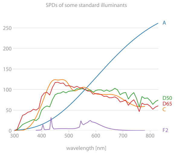
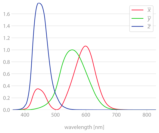
Illuminants, observers, white points
| Illuminants | CIE 1931 Observer |
|---|---|
 |
 |
import coloria
import matplotlib.pyplot as plt

illu = coloria.illuminants.d65()
plt.plot(illu.lmbda_nm, illu.data)
plt.xlabel("wavelength [nm]")
plt.show()
The following illuminants are provided:
- Illuminant A ("indoor light",
coloria.illuminants.a(resolution_in_nm)) - Illuminant C (obsolete, "North sky daylight",
coloria.illuminants.c()) - Illuminants D ("natural daylight",
coloria.illuminants.d(nominal_temp)orcoloria.illuminants.d65()etc.) - Illuminant E (equal energy,
coloria.illuminants.e()) - Illuminant series F ("fluorescent lighting",
coloria.illuminants.f2()etc.)
Observers:
- CIE 1931 Standard 2-degree observer (
coloria.observers.coloria.observers.cie_1931_2()) - CIE 1964 Standard 10-degree observer (
coloria.observers.coloria.observers.cie_1964_10())
Color appearance models
Color appearance models (CAMs) predicts all kinds of parameters in color perception, e.g., lightness, brightness, chroma, colorfulness, saturation etc. Since these values depend on various factors, such as the surrouning, the models are initialized with various different parameters.
CAMs can be used to construct color spaces (see below).
The color appearance models available in coloria are
-
CIECAM02 / CAM02-UCS
import coloria

ciecam02 = coloria.cam.CIECAM02(
    surround_type="average",  # or dim, dark
    background_luminance_percent=20,
    adapting_luminance_cd_m2=100,
)

xyz = [19.31, 23.93, 10.14]
corr = ciecam02.from_xyz100(xyz)
# then work with those values:
corr.lightness
corr.brightness
corr.chroma
corr.hue_composition
corr.hue_angle_degrees
corr.colorfulness
corr.saturation
-
CAM16 / CAM16-UCS
import coloria

cam16 = coloria.cam.CAM16("average", 20, 100)
-
ZCAM
import coloria

cam16 = coloria.cam.ZCAM("average", 20, 100, 20)
Color coordinates and spaces
Color coordinates are handled as NumPy arrays or as ColorCoordinates, a thin
wrapper around the data that retains the color space information and has some
handy helper methods. Color spaces can be instantiated from the classes in
coloria.cs, e.g.,
import coloria

coloria.cs.CIELAB()
Most methods that accept such a colorspace also accept a string, e.g.,
cielab.
As an example, to interpolate two sRGB colors in OKLAB, and return the sRGB:
from coloria.cs import ColorCoordinates

# you can also plug in large numpy arrays instead of two lists here
c0 = ColorCoordinates([1.0, 1.0, 0.0], "srgb1")  # yellow
c1 = ColorCoordinates([0.0, 0.0, 1.0], "srgb1")  # blue

# naive interpolation gives [0.5, 0.5, 0.5], a mid gray

# convert to OKLAB
c0.convert("oklab")
c1.convert("oklab")

# interpolate
c2 = (c0 + c1) * 0.5

c2.convert("srgbhex", mode="clip")

print(c2.color_space)
print(c2.data)
<coloria color space sRGB-hex>
#6cabc7
All color spaces implement the two methods
vals = colorspace.from_xyz100(xyz)
xyz = colorspace.to_xyz100(vals)
for conversion from and to XYZ100. Adding new color spaces is as easy as writing a class that provides those two methods. The following color spaces are already implemented:
-
XYZ (
coloria.cs.XYZ(100), the parameter determining the scaling) -
xyY (
coloria.cs.XYY(100), the parameter determining the scaling ofY) -
sRGB (
coloria.cs.SRGBlinear(),coloria.cs.SRGB1(),coloria.cs.SRGB255(),coloria.cs.SRGBhex()) -
HSL and HSV (
coloria.cs.HSL(),coloria.cs.HSV()) These classes also have the two methodsfrom_srgb1() to_srgb1()for direct conversion from and to standard RGB.
-
CIE 1960 UCS (
coloria.cs.CIE1960UCS()), 1960 -
CIEUVW (
coloria.cs.CIEUVW()), 1964 -
CIELAB (
coloria.cs.CIELAB()), 1976 -
CIELUV (
coloria.cs.CIELUV()), 1976 -
RLAB (
coloria.cs.RLAB()), 1993 -
IPT (
coloria.cs.IPT()), 1998 -
DIN99 and its variants DIN99{b,c,d} (
coloria.cs.DIN99()), 1999 -
CAM02-UCS, 2002
import coloria

cam02 = coloria.cs.CAM02("UCS", "average", 20, 100)
The implementation contains a few improvements over the CIECAM02 specification (see here).
-
CAM16-UCS, 2016
import coloria

cam16ucs = coloria.cs.CAM16UCS("average", 20, 100)
The implementation contains a few improvements over the CAM16 specification (see here).
-
SRLAB2 (
coloria.cs.SRLAB2()) -
Jzazbz (
coloria.cs.JzAzBz()), 2017 -
OkLCh (
coloria.cs.OKLCH()), 2020
All methods in coloria are fully vectorized, i.e., computation is really fast.
Color difference formulas
coloria implements the following color difference formulas:
- CIE76
coloria.diff.cie76(lab1, lab2)
- CIE94
coloria.diff.cie94(lab1, lab2)
- CIEDE2000
coloria.diff.ciede2000(lab1, lab2)
- CMC l:c
coloria.diff.cmc(lab1, lab2)
Chromatic adaptation transforms
coloria implements the following CATs:
- von Kries
cat, cat_inv = coloria.cat.von_kries(whitepoint_source, whitepoint_destination)
xyz1 = cat @ xyz0
- Bradford (
coloria.cat.bradford) - sharp (
coloria.cat.sharp) - CMCCAT2000 (
coloria.cat.cmccat2000) - CAT02 (
coloria.cat.cat02) - CAT16 (
coloria.cat.cat16) - Bianco-Schettini (
coloria.cat.bianco_schettini)
Gamut visualization
coloria provides a number of useful tools for analyzing and visualizing color spaces.
sRGB gamut
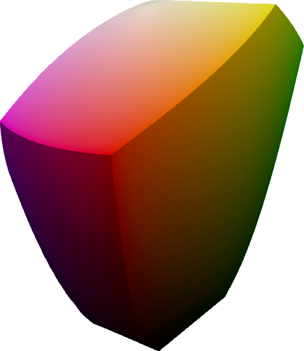
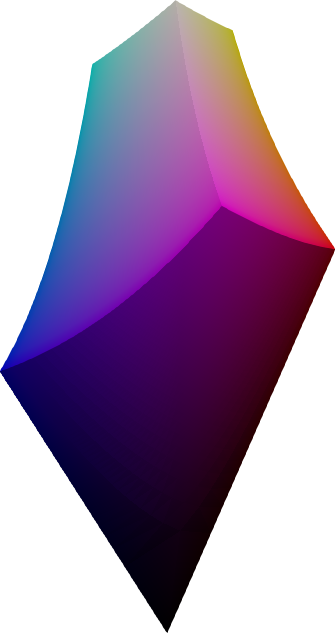
| CIELAB | CAM16-UCS | Oklab |
|---|---|---|
 |
 |
 |
 |
 |
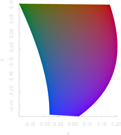 |
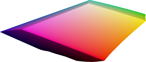
The sRGB gamut is a perfect cube in sRGB space, and takes curious shapes when translated into other color spaces. The above images show the sRGB gamut in different color spaces.
import coloria

p = coloria.plot_rgb_gamut(
    "cielab",  # or coloria.cs.CIELAB()
    n=51,
    show_grid=True,
)
p.show()
For more visualization options, you can store the sRGB data in a file
import coloria

coloria.save_rgb_gamut("srgb.vtk", "cielab", n=51)
# all formats supported by https://github.com/coloria-dev/meshio
and open it with a tool of your choice. See here for how to open the file in ParaView.
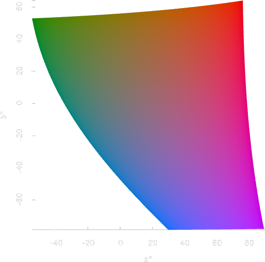
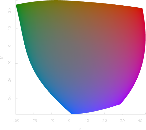
For lightness slices of the sRGB gamut, use
import coloria

p = coloria.plot_rgb_slice("cielab", lightness=50.0, n=51)
p.show()
# or
# p.screenshot("screenshot.png")
Surface color gamut
 |
 |
 |
|---|---|---|
| XYZ | CIELAB | CAM16-UCS |
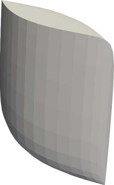
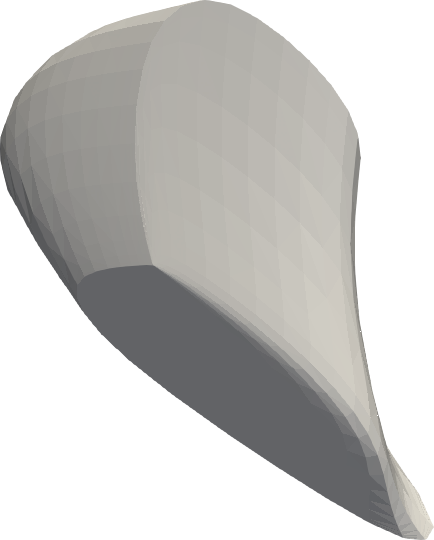
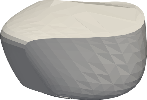
Same as above, but with the surface color gamut visible under a given illuminant.
import coloria

illuminant = coloria.illuminants.d65()
observer = coloria.observers.cie_1931_2()

p = coloria.plot_surface_gamut(
    "xyz100",  # or coloria.cs.XYZ(100)
    observer,
    illuminant,
)
p.show()
The gamut is shown in grey since sRGB screens are not able to display the colors anyway.
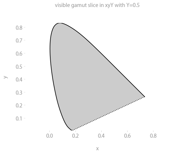
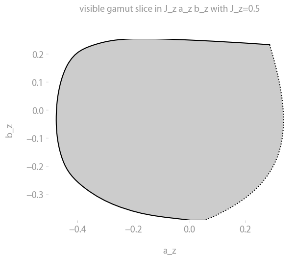
The visible gamut
| xyY | JzAzBz | Oklab |
|---|---|---|
 |
 |
 |
 |
 |
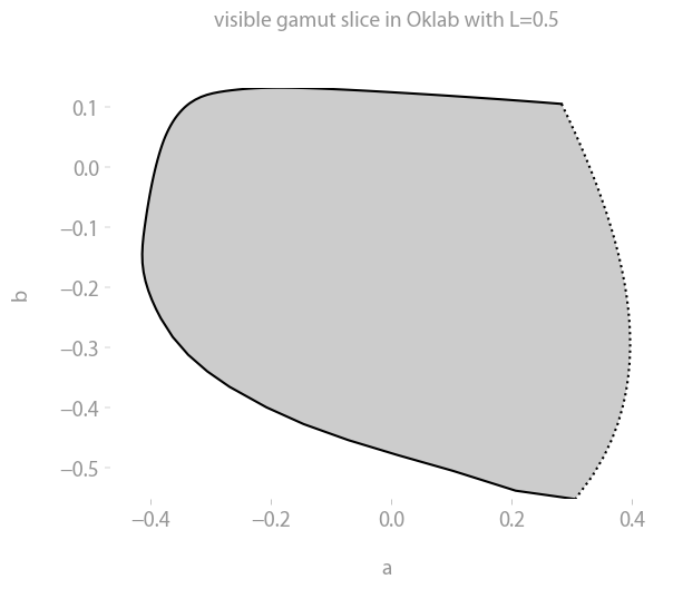 |
Same as above, but with the gamut of visible colors up to a given lightness Y.
import coloria

observer = coloria.observers.cie_1931_2()

colorspace = coloria.cs.XYZ(100)

p = coloria.plot_visible_gamut(colorspace, observer, max_Y1=1)
p.show()
The gamut is shown in grey since sRGB screens are not able to display the colors anyway.
For slices, use
import coloria

plt = coloria.plot_visible_slice("cielab", lightness=0.5)
plt.show()
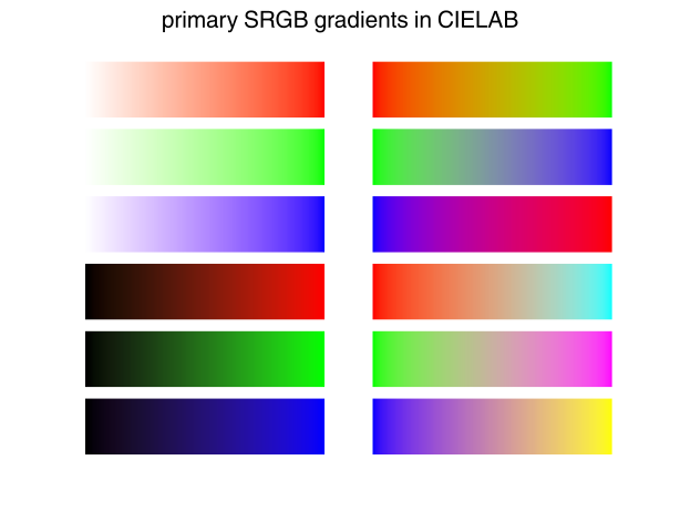
Color gradients
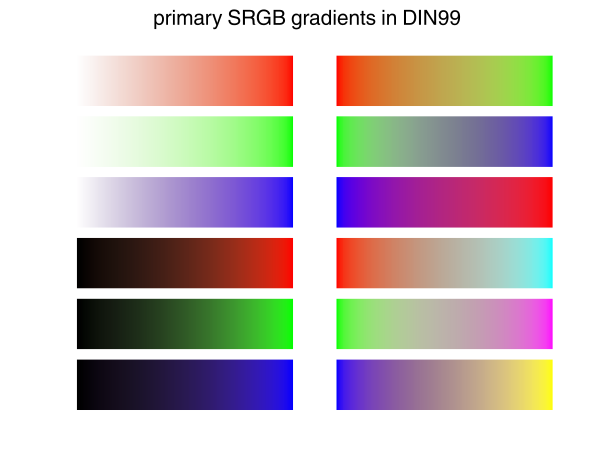
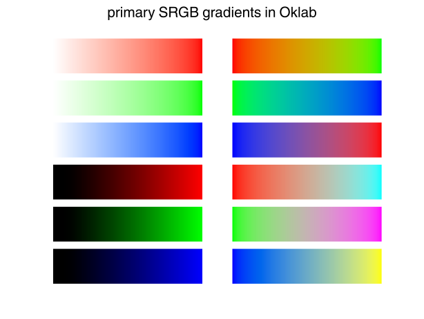
With coloria, you can easily visualize the basic color gradients of any color space. This may make defects in color spaces obvious, e.g., the well-known blue-distortion of CIELAB and related spaces. (Compare with the hue linearity data below.)
import coloria

plt = coloria.plot_primary_srgb_gradients("cielab")
plt.show()
 |
 |
 |
|---|---|---|
| CIELAB | DIN99 | OKLAB |
Experimental data
coloria contains lots of experimental data sets some of which can be used to assess certain properties of color spaces. Most data sets can also be visualized.
Color differences
 |
 |
 |
|---|---|---|
| xyY | CIELAB | CAM16 |
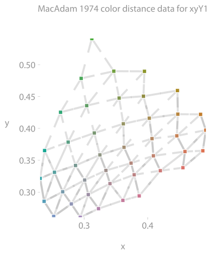
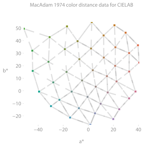
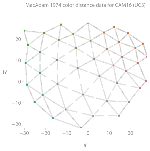
Color difference data from MacAdam (1974). The above plots show the 43 color pairs that are of comparable lightness. The data is matched perfectly if the facing line stubs meet in one point.
import coloria

data = coloria.data.MacAdam1974()

cs = coloria.cs.CIELAB

plt = data.plot(cs)
plt.show()
print(coloria.data.MacAdam1974().stress(cs))
24.54774029343344
The same is available for
coloria.data.BfdP()
coloria.data.Leeds()
coloria.data.RitDupont()
coloria.data.Witt()

coloria.data.COMBVD()  # a weighted combination of the above
Munsell
 |
 |
 |
|---|---|---|
| xyY | CIELAB | CAM16 |
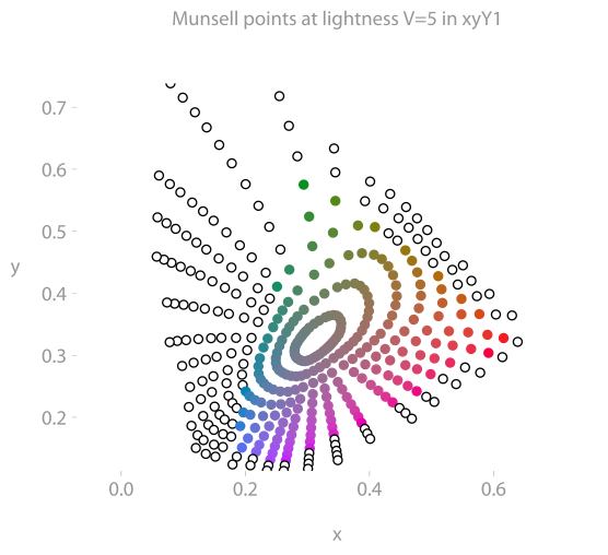
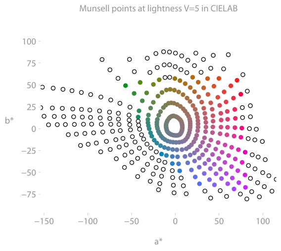
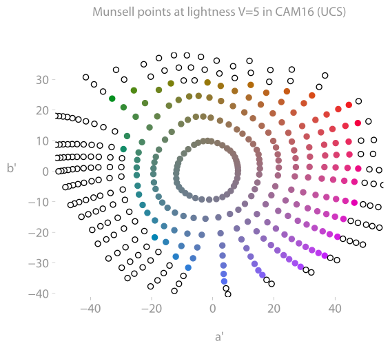
Munsell color data is visualized with
import coloria

cs = coloria.cs.CIELUV
plt = coloria.data.Munsell().plot(cs, V=5)
plt.show()
To retrieve the Munsell data in xyY format, use
import coloria

munsell = coloria.data.Munsell()

# munsell.h
# munsell.V
# munsell.C
# munsell.xyy
Ellipses
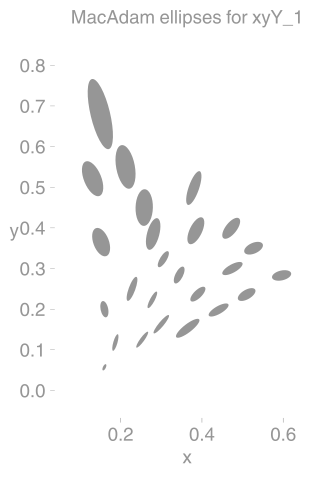
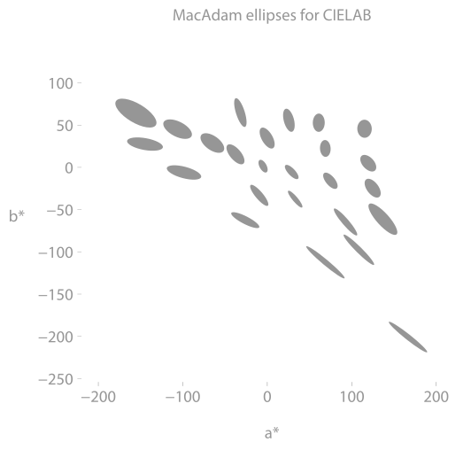
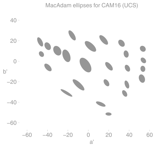
MacAdam ellipses (1942)
 |
 |
 |
|---|---|---|
| xyY (at Y=0.4) | CIELAB (at L=50) | CAM16 (at L=50) |
The famous MacAdam ellipses (from this article) can be plotted with
import coloria

cs = coloria.cs.CIELUV
plt = coloria.data.MacAdam1942(50.0).plot(cs)
plt.show()
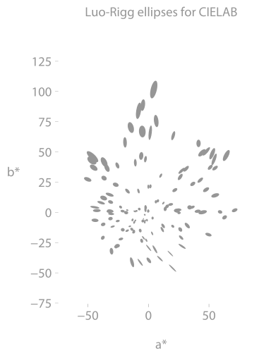
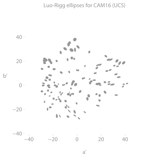
The better the colorspace matches the data, the closer the ellipses are to circles of the same size.
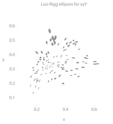
Luo-Rigg ellipses
 |
 |
 |
|---|---|---|
| xyY | CIELAB | CAM16 |
Likewise for Luo-Rigg.
import coloria

# xyy = coloria.cs.XYY(100)
# coloria.data.LuoRigg(8).show(xyy, 0.4)
# coloria.data.LuoRigg(8).savefig("luo-rigg-xyy.png", xyy, 0.4)

cieluv = coloria.cs.CIELUV()
plt = coloria.data.LuoRigg(8).plot(cieluv, 50)
plt.show()
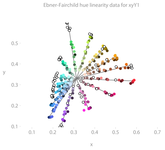
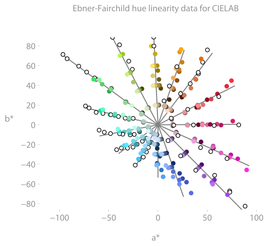
Hue linearity
Ebner-Fairchild
 |
 |
 |
|---|---|---|
| xyY | CIELAB | CAM16 |
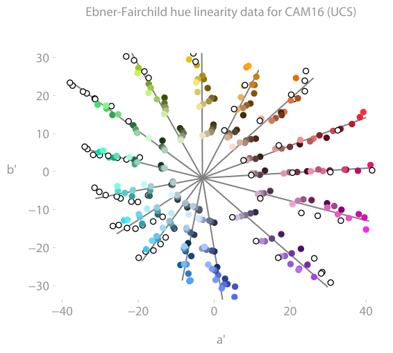
For example
import coloria

colorspace = coloria.cs.JzAzBz
plt = coloria.data.EbnerFairchild().plot(colorspace)
plt.show()
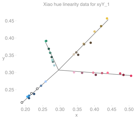
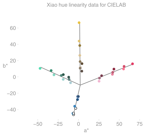
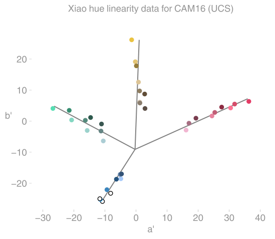
shows constant-hue data from the Ebner-Fairchild experiments in the hue-plane of some color spaces. (Ideally, all colors in one set sit on a line.)
Hung-Berns
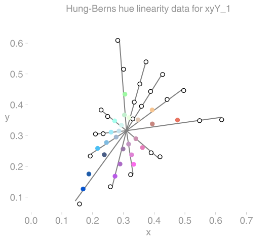
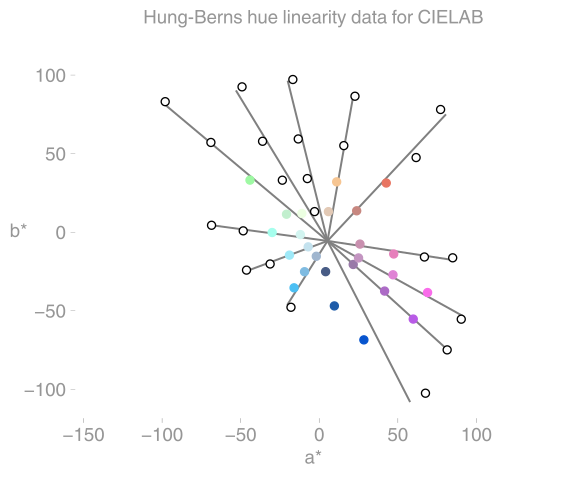
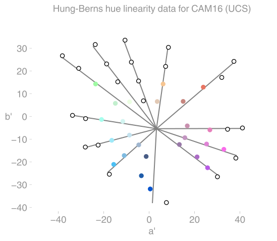
Likewise for Hung-Berns:
 |
 |
 |
|---|---|---|
| xyY | CIELAB | CAM16 |
Note the dark blue distortion in CIELAB and CAM16.
import coloria

colorspace = coloria.cs.JzAzBz
plt = coloria.data.HungBerns().plot(colorspace)
plt.show()
Xiao et al.
Likewise for Xiao et al.:
 |
 |
 |
|---|---|---|
| xyY | CIELAB | CAM16 |
import coloria

colorspace = coloria.cs.CIELAB
plt = coloria.data.Xiao().plot(colorspace)
plt.show()
Lightness
Fairchild-Chen
 |
 |
 |
|---|---|---|
| xyY | CIELAB | CAM16 |
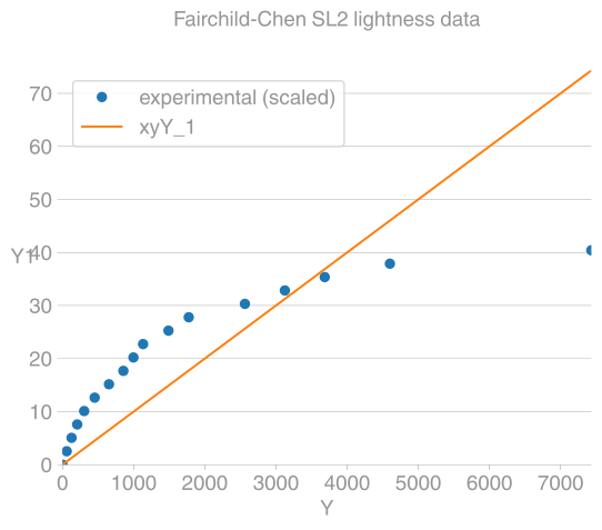
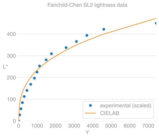
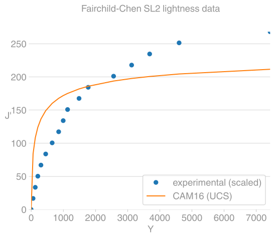
Lightness experiment by Fairchild-Chen.
import coloria

cs = coloria.cs.CIELAB
plt = coloria.data.FairchildChen("SL2").plot(cs)
plt.show()
Articles
1 maintainer

Metadata
1 maintainer
Release files for coloria 0.14.12
For a detailed explanation of source distributions (sdists) and built distributions (wheels), please see the package formats documentation.
Built distributions (wheels)
| File | Reset | |||
|---|---|---|---|---|
| coloria-0.14.12-cp314-none-any.whl | CPython 3.14 | none | any | Details |
| coloria-0.14.12-cp313-none-any.whl | CPython 3.13 | none | any | Details |
| coloria-0.14.12-cp312-none-any.whl | CPython 3.12 | none | any | Details |
| coloria-0.14.12-cp311-none-any.whl | CPython 3.11 | none | any | Details |
| coloria-0.14.12-cp310-none-any.whl | CPython 3.10 | none | any | Details |
Total release size: 4.8 MB
Release files / coloria-0.14.12-cp314-none-any.whl
| Download URL | coloria-0.14.12-cp314-none-any.whl |
|---|---|
| Size | 988.6 kB |
| Tags | CPython 3.14 |
|
SHA-256 checksum How to use checksums |
dc03398e11c38619fce5f9ea2b22a4e0aa2f9d95cd361df6a9847db316682085
|
|
BLAKE2b-256 checksum How to use checksums |
73f3fff8739a4bdae5c7eb7ef3f38529ffff1bf9bd0a323fe6e219520328d61a
|
| Upload date | |
|
Uploaded using Trusted Publishing? What is trusted publishing? |
Yes |
| Uploaded via |
twine/6.1.0 CPython/3.13.12
|
Provenance
Provenance describes where a file came from. On PyPI, provenance is shared via attestations, which provide a verifiable record of the build or publishing details. View details, limitations and caveats.


PyPI Publish Attestation
PyPI verified that this artifact, at this checksum, originated from the publisher listed below.
Signed by GitHub Actions, verified by PyPI on May 18, 2026.
Transparency logRelease files / coloria-0.14.12-cp313-none-any.whl
| Download URL | coloria-0.14.12-cp313-none-any.whl |
|---|---|
| Size | 969.4 kB |
| Tags | CPython 3.13 |
|
SHA-256 checksum How to use checksums |
ebe0f2713fc62741ef169e8bc04597b45d56f8ebac6c732abcb92568c0062a00
|
|
BLAKE2b-256 checksum How to use checksums |
2294c3c5d9aa994c3d566307cd802d60b9b415061f84f8c8d114c6316d96d2bd
|
| Upload date | |
|
Uploaded using Trusted Publishing? What is trusted publishing? |
Yes |
| Uploaded via |
twine/6.1.0 CPython/3.13.12
|
Provenance
Provenance describes where a file came from. On PyPI, provenance is shared via attestations, which provide a verifiable record of the build or publishing details. View details, limitations and caveats.
PyPI Publish Attestation
PyPI verified that this artifact, at this checksum, originated from the publisher listed below.
Signed by GitHub Actions, verified by PyPI on May 18, 2026.
Transparency logRelease files / coloria-0.14.12-cp312-none-any.whl
| Download URL | coloria-0.14.12-cp312-none-any.whl |
|---|---|
| Size | 969.5 kB |
| Tags | CPython 3.12 |
|
SHA-256 checksum How to use checksums |
a5c844412241173223cdd7fe8a9f84a2d12552c45de960ee6f97114a5f37263d
|
|
BLAKE2b-256 checksum How to use checksums |
184c37ed6fa72f00573ee38077b8944903d9a3d6fc2e6676cef6cd05cc5ca731
|
| Upload date | |
|
Uploaded using Trusted Publishing? What is trusted publishing? |
Yes |
| Uploaded via |
twine/6.1.0 CPython/3.13.12
|
Provenance
Provenance describes where a file came from. On PyPI, provenance is shared via attestations, which provide a verifiable record of the build or publishing details. View details, limitations and caveats.
PyPI Publish Attestation
PyPI verified that this artifact, at this checksum, originated from the publisher listed below.
Signed by GitHub Actions, verified by PyPI on May 18, 2026.
Transparency logRelease files / coloria-0.14.12-cp311-none-any.whl
| Download URL | coloria-0.14.12-cp311-none-any.whl |
|---|---|
| Size | 998.0 kB |
| Tags | CPython 3.11 |
|
SHA-256 checksum How to use checksums |
386b1d1c699e4de5b4758ae460b80e6779eeeb37a0e9df00123e9744974b67f7
|
|
BLAKE2b-256 checksum How to use checksums |
c9d3c795eb14e981b8331aadd5535f838f21040c9b714b991f224c5406d8b5af
|
| Upload date | |
|
Uploaded using Trusted Publishing? What is trusted publishing? |
Yes |
| Uploaded via |
twine/6.1.0 CPython/3.13.12
|
Provenance
Provenance describes where a file came from. On PyPI, provenance is shared via attestations, which provide a verifiable record of the build or publishing details. View details, limitations and caveats.
PyPI Publish Attestation
PyPI verified that this artifact, at this checksum, originated from the publisher listed below.
Signed by GitHub Actions, verified by PyPI on May 18, 2026.
Transparency logRelease files / coloria-0.14.12-cp310-none-any.whl
| Download URL | coloria-0.14.12-cp310-none-any.whl |
|---|---|
| Size | 825.4 kB |
| Tags | CPython 3.10 |
|
SHA-256 checksum How to use checksums |
e4bde1bd948a717bf7dae8ca87d261021da49c10a7adb83c82cc89aaf3113bb6
|
|
BLAKE2b-256 checksum How to use checksums |
7ffef97a0406260342d804cbb20b6656edb60e09a43a313ddc9ea83ad700b47d
|
| Upload date | |
|
Uploaded using Trusted Publishing? What is trusted publishing? |
Yes |
| Uploaded via |
twine/6.1.0 CPython/3.13.12
|
Provenance
Provenance describes where a file came from. On PyPI, provenance is shared via attestations, which provide a verifiable record of the build or publishing details. View details, limitations and caveats.
PyPI Publish Attestation
PyPI verified that this artifact, at this checksum, originated from the publisher listed below.
Signed by GitHub Actions, verified by PyPI on May 18, 2026.
Transparency log













