





ComPyTools is an open source (MIT) Python package for working with equation of state (EoS) tables in the CompOSE ("CompStar Online Supernova Equations of State") format. It provides tools to read, write and analyse CompOSE tables within Python workflows, leveraging astropy for data tables, units and metadata.
ComPyTools allows the user to:
- Read in CompOSE cold or general purpose EoS tables,
- Create interpolated tables from cold or general purpose EoSs via a Python interface to the CompOSE code,
- Produce cold EoS tables in the CompOSE format for those who wish to contribute their own EoS to the CompOSE database.
Quick Example 1: Reading CompOSE tables
import tempfile
import matplotlib.pyplot as plt

from compytools import EoS
from compytools.download import CompOSEDownloader

# Download sample data into temporary directory
# for purposes of this example
tmpdir = tempfile.TemporaryDirectory()
downloader = CompOSEDownloader.from_eosname('PCP(BSk22)', tmpdir.name)
downloader.get()

bsk22 = EoS.from_compose(tmpdir.name)

# View the data in tabular form
bsk22.thermo.pprint(max_width=-1)

# View column descriptions
print(bsk22.thermo.info)

nb = bsk22.params.nb.grid_points
# Q1 corresponds to the ratio p/nb
pressure = bsk22.thermo['Q1'] * nb
plt.loglog(nb, pressure)
plt.grid()

plt.xlabel(r'$n_{B}$ [fm$^{-3}$]')
plt.ylabel(r'$p$ [MeV fm$^{-3}$]')
plt.show()
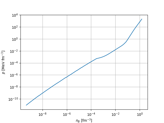
Quick Example 2: Create interpolated tables from cold CompOSE data
import tempfile

from compytools import (
    GridSettings,
    Interface,
    summarise
)

from compytools.download import CompOSEDownloader

# Download a sample table
tmpdir = tempfile.TemporaryDirectory()
getter = CompOSEDownloader.from_eosname('PCP(BSk22)', tmpdir.name)
getter.get()

# Summarise the grid parameters and available
# thermodynamic quantities
summarise(tmpdir.name, tables='thermo')
┏━━━━━━━━━━━━━━━━━┳━━━━━━━━━━━━━━━━━━━━━━━━━━━━━━━━━━━━━━━━━━━━━━━━┳━━━━━━━━━━━━━━━┓
┃ Quantity Number ┃ Quantity                                       ┃ Unit          ┃
┡━━━━━━━━━━━━━━━━━╇━━━━━━━━━━━━━━━━━━━━━━━━━━━━━━━━━━━━━━━━━━━━━━━━╇━━━━━━━━━━━━━━━┩
│ 1               │ total pressure                                 │ 1.0 MeV / fm3 │
│ 2               │ total entropy per baryon                       │               │
│ 3               │ shifted baryon chemical potential              │ MeV           │
│ 4               │ charge chemical potential                      │ MeV           │
│ 5               │ lepton chemical potential                      │ MeV           │
│ 6               │ Scaled free energy per baryon                  │               │
│ 7               │ Scaled internal energy per baryon              │               │
│ 8               │ Scaled enthalpy per baryon                     │               │
│ 9               │ Scaled free enthalpy per baryon                │               │
│ 18              │ isothermal compressibility                     │ fm3 / MeV     │
│ 20              │ Free energy per baryon                         │ MeV           │
│ 21              │ Energy per baryon (with rest mass              │ MeV           │
│                 │ contribution)                                  │               │
│ 22              │ enthalpy per baryon                            │ MeV           │
│ 23              │ free enthalpy per baryon                       │ MeV           │
│ 24              │ Energy density                                 │ 1.0 MeV / fm3 │
└─────────────────┴────────────────────────────────────────────────┴───────────────┘
# 1. Define the grid in baryon number density for the interpolation
nbgrid = GridSettings(
    # Min. and max. grid point values
    min=1.e-7,
    max=1.0,
    # interpolation order
    order=2,
    # Num. of points
    npoints=200,
    # Choose grid on log scale
    logscale=True
)

# 2. Set up the CompOSE interface
interface = Interface(
    # Directory containing the tables
    eospath=tmpdir.name,
    # Grid settings for baryon number density
    nbconfig=nbgrid,
    # Values defining pressure (1) and energy density (24)
    # given in the summary table above
    thermo_choice=[1, 24]
)

# 3. Run the interface and display the table.
# The table is saved to the same location as the
# CompOSE tables.
table = interface.run()
table.pprint()
Quick Example 3: Create mandatory CompOSE tables for a cold EoS
import os
import tempfile

from urllib.request import urlretrieve

import numpy as np

from compytools import (
    EoS,
    Grid,
    GridData,
    Thermo,
    ThermoData,
    NeutronStar,
    NeutronStarData,
    Nucleons
)

from compytools.constants import (
    DIMENSIONLESS,
    DYN_PER_CM2,
    G_PER_CM3,
    GRAM,
    MEV,
    PERFM3
)

# Download sample data to be converted into CompOSE format
tmpdir = tempfile.TemporaryDirectory()
eos_file = "eos_akmalpr.d"
eos_url = "https://gitlab.in2p3.fr/lpc-caen/compytools/-/raw/main/tests/inputs/lorene/"

source = os.path.join(eos_url, eos_file)
dest = os.path.join(tmpdir.name, eos_file)

urlretrieve(source, dest)

# Load the data
nbgrid, rho, p = np.loadtxt(
    dest,
    # Ignore file's header info
    skiprows=9,
    usecols=(1, 2, 3),
    unpack=True
)

# Prepare the grid parameter data
# 1. Enter the grid parameter data with units
grid_data = GridData(
    # Temperature grid points in MeV. Zero for a cold EoS
    t=np.array([0.0]) << MEV,
    # Baryon number density in 1/fm^3
    nb=nbgrid << PERFM3,
    # Charge fraction (no units). Zero for a cold EoS
    yq=np.array([0.0]) << DIMENSIONLESS
)

# 2. Convert into tabular format
grid_params = Grid.from_dataset(grid_data)

# Prepare the thermodynamic quantities
# 1. Nucleon masses
nucleons = Nucleons(
    mn=1.6749286e-24 << GRAM,
    mp=1.6726231e-24 << GRAM,
    # Indicates that leptons are considered (0 otherwise)
    has_leptons=1
)

# 2. Enter thermodynamic quantities with units
thermo_data = ThermoData(
    grid_params=grid_params,
    nucleons=nucleons,
    pressure=p << DYN_PER_CM2,
    entropy_density=np.zeros(nbgrid.size) << PERFM3,
    charge_chemical_potential=np.zeros(nbgrid.size) << MEV,
    lepton_chemical_potential=np.zeros(nbgrid.size) << MEV,
    # Free and internal energy densities are equal for a cold EoS
    free_energy_density=rho << G_PER_CM3,
    internal_energy_density=rho << G_PER_CM3,
)

# 3. Convert data into tabular form
thermo = Thermo.from_dataset(thermo_data)

# Calculate the static neutron star properties
# 1. Compute the data
ns_data = NeutronStarData(
    grid_params=grid_params,
    thermo=thermo
)

# 2. Convert to tabulated form
mr = NeutronStar.from_dataset(ns_data)

# Combine the tables and write the CompOSE files
myeos = EoS(
    params=grid_params,
    thermo=thermo,
    mr=mr
)

# Write the files to your current working directory
myeos.to_compose('./')
Documentation
Full documentation, including installation instructions, a tutorial and an API reference can be found on the ComPyTools web page.
Requirements
ComPyTools requires at least Python 3.12 along with the following Python packages, which will be installed automatically via the steps outlined in the Installation section:
- Astropy: for displaying data in tabular form and to attach metadata and units to the data. We also use physical constants defined within astropy,
- lalsuite: for solving the Tolman-Oppenheimer-Volkoff equations to calculate neutron star static properties,
- Matplotlib: for plotting EoS data,
- Pandas: for writing out tabulated data into text files,
- PDG: for accessing particle masses via the Particle Data Group (PDG) database,
- requests: for downloading sample data,
- Rich: for log output and tabulating metadata information,
- Scipy: for performing integration, optimization and interpolation tasks.
Additional packages are also needed to install and build ComPyTools:
- CompOSE: a set of Fortran routines for computing the interpolated tables. This is included as part of the ComPyTools package,
- cmake and make: for compiling the CompOSE Fortran routines,
- gfortran: compiler for the Fortran routines,
- micromamba or conda: for creating the software environment within which to install ComPyTools,
- tectonic: required when creating the CompOSE PDF datasheet describing a contributor's EoS.
Installation
For Linux, MacOS or WSL for Windows, install micromamba (recommended for a more optimized, drop-in replacement of conda) with
"${SHELL}" <(curl -L micro.mamba.pm/install.sh)
and create the micromamba environment in order to install the build and compilation tools:
micromamba create -n compytools-env -c conda-forge python=3.12 cmake make gfortran tectonic
Activate the environment with
micromamba activate compytools-env
Then, install ComPyTools with pip:
pip install compytools
This will also compile CompOSE on your machine. You can test the installation with:
python -c "import compytools"
Further details can be found on the installation instructions.
License
ComPyTools is released under the MIT license.
Acknowledgements
The development of ComPyTools has been partially supported by the French Centre National de la Recherche Scientifique (CNRS) International Research Project (IRP) "Origine des éléments lourds dans l'univers: Astres Compacts et Nucléosynthèse (ACNu)".
We also acknowledge contributions from the CompOSE core development team and members of the LuTH-Caen group within the Virgo collaboration.
Contributing and contact
ComPyTools is a community project. We therefore welcome and appreciate any comments that you may have to improve the tool. Suggestions or bug reports can be communicated to Philip Davis at the following email address: davis@lpccaen.in2p3.fr, or by opening an issue.
1 maintainer

Metadata
1 maintainer
Release files for compytools 0.2.0
For a detailed explanation of source distributions (sdists) and built distributions (wheels), please see the package formats documentation.
Source distribution (sdist)
| File | Size | Uploaded | |
|---|---|---|---|
| compytools-0.2.0.tar.gz | 308.9 kB | Details |
Release files / compytools-0.2.0.tar.gz
| Download URL | compytools-0.2.0.tar.gz |
|---|---|
| Size | 308.9 kB |
| Tags | Source |
|
SHA-256 checksum How to use checksums |
583fff0a0b67bf8a4355eb984a4a83cfcbeb5f63bbddcdcbb2872cbb4c515c8a
|
|
BLAKE2b-256 checksum How to use checksums |
08bd78558095a8a1332ae05898ff3bab8308700288cf9a8dea30f8185650cf34
|
| Upload date | |
|
Uploaded using Trusted Publishing? What is trusted publishing? |
No |
| Uploaded via |
twine/7.0.0 CPython/3.12.15
|














