
Concept Benchmark


Concept Benchmark is a Python package for benchmarking concept bottleneck models (CBMs). A CBM predicts interpretable concepts from the input (e.g., "has pointy feet") and the label from the concepts, so a user can inspect and correct the concepts at test time. Very few datasets include concept labels, which makes it hard to tell where these models work and why they fail.
We provide dataset generators that produce labeled data from a known concept-to-label rule while varying modality, concept granularity, annotation quality and missingness, and build one benchmark on them for each of the two use cases where CBMs provide unique value:
- Robot Classification — decision support, measured by the gain over a black-box model when a human corrects the concepts. Images or text.
- Sudoku Validation — automation, measured by the human work saved when the model answers routine boards and defers the rest. A board is valid only if all 27 concepts hold, so one wrong concept fails it.
Table of Contents
- Installation
- Quick Start
- Benchmarks
- Benchmark Your Own Model
- Interventions and Alignment
- Reproducing the Paper
- Citation
Installation
The package requires the cairo graphics library. Install it first:
# macOS
brew install cairo pkg-config

# Ubuntu / Debian
sudo apt-get install libcairo2-dev pkg-config python3-dev

# Fedora / RHEL
sudo dnf install cairo-devel pkg-config python3-devel
Then install the package:
pip install concept-benchmark
Dataset generation, metrics, and plots work out of the box with pip install. Model training and interventions (experiments/ package and the pipelines in scripts/) require cloning the repo:
git clone https://github.com/ustunb/concept-benchmark.git
cd concept-benchmark
uv sync
Verify the installation:
python3 -c "import concept_benchmark; print(concept_benchmark.__version__)"
Optional: CEM, ProbCBM, and ECBM
The repo also trains three other architectures: CEM and ProbCBM from the official mateoespinosa/cem package, and ECBM, which is included and follows the authors' code. Install the CEM package with
./scripts/install_cem_repo.sh
or by hand:
git clone https://github.com/mateoespinosa/cem.git third_party/cem
python -m pip install "pytorch-lightning>=1.6,<2.0" "torchmetrics<1.0"
python -m pip install -r third_party/cem/requirements.txt
python -m pip install -e third_party/cem
Then pass --cbm-family cem, probcbm or ecbm to the robot or sudoku pipeline (the text pipeline trains the CBM only). Their settings (cem_emb_size, training_mode, probcbm_n_samples_inference, …) are fields of the config; see docs/installation.md.
Quick Start
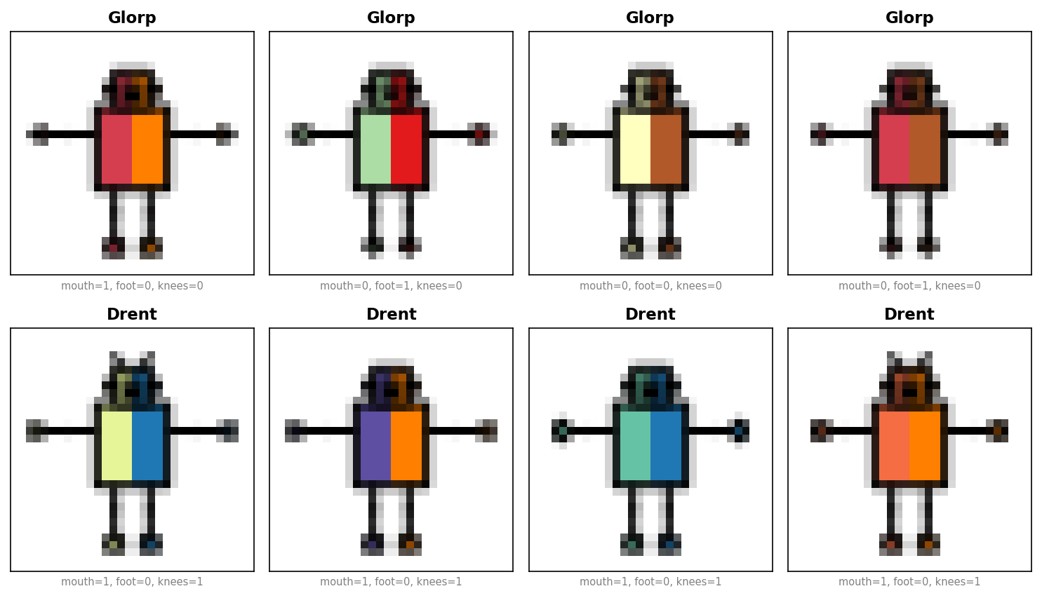
Robot — classify fictional robots (Glorps vs. Drents) from body features:
from concept_benchmark.robots import DatasetGenerator

dataset = DatasetGenerator(
    seed=1014,
    concept_preset="foot_subtypes",  # expand foot_shape into subtypes (default: "ground_truth")
    render_images=True,              # set False to skip rendering for quick exploration
).generate_splits()                  # the train/val/test split of the paper

print(dataset.train.C.shape)   # (3800, 12) — concept annotations
print(dataset.train.concepts)
# ['head_shape', 'body_shape', 'has_knees', 'has_antennae', 'ears_shape',
#  'mouth_type', 'foot_shape_flat_trapezoid', 'foot_shape_flat_square',
#  'foot_shape_flat_5sided', 'foot_shape_pointy_rounded',
#  'foot_shape_pointy_square', 'foot_shape_pointy_4sided']
generate() returns the unsplit dataset with every concept, for you to drop concepts and split as you choose (see Post-processing).
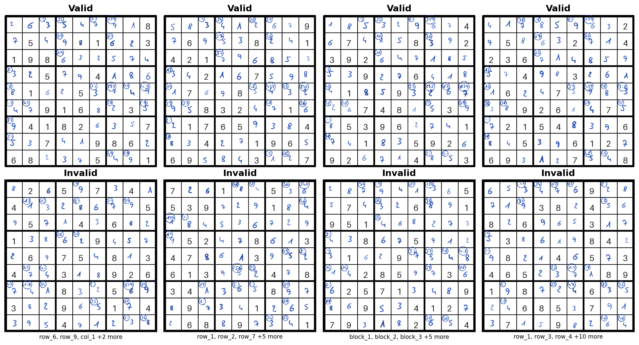
Sudoku — determine whether a 9×9 board is valid. 27 concepts capture row, column, and block validity:
from concept_benchmark.sudoku import DatasetGenerator

dataset = DatasetGenerator(
    seed=171,             # reproducibility
    n_boards=1000,        # number of boards
    max_cell_swaps=9,     # corruptions applied to each invalid board, 1 to 9 (each swaps or duplicates digits)
    valid_board_ratio=0.5,  # fraction of valid boards
    render_images=False,  # set True to generate board images (slower)
).generate_splits()       # 60/20/20, stratified on the label

print(dataset.train.C.shape)   # (600, 27) — 27 concept annotations
print(dataset.train.concepts)  # ['row_valid_1', 'row_valid_2', ..., 'block_valid_9']
The datasets of the paper are also on the Hugging Face Hub, if you prefer to download them (robots-true-concepts, robots-human-concepts, sudoku):
# pip install datasets
from datasets import load_dataset
ds = load_dataset("juliannski/robots-human-concepts")
For complete walkthroughs including training and evaluation, see examples/robot_pipeline_example.py and examples/sudoku_pipeline_example.py.
Benchmarks
Robot Classification
Parameters
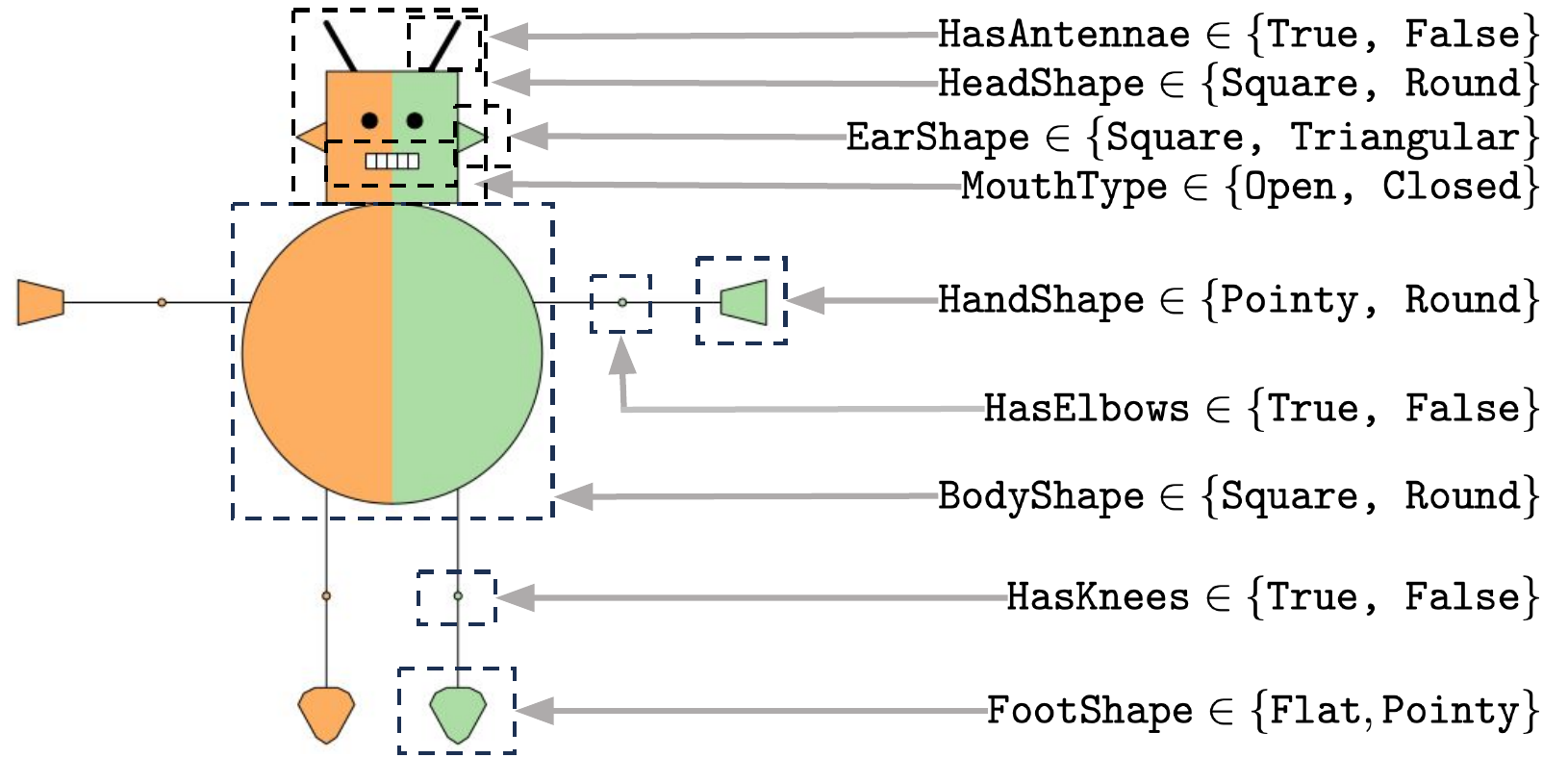
All parameters are keyword arguments of DatasetGenerator (from concept_benchmark.robots). The ones most users set:
from concept_benchmark.robots import DatasetGenerator

dataset = DatasetGenerator(
    seed=1014,
    data_type="image",               # or "text"
    concept_preset="foot_subtypes",  # "ground_truth" (7 concepts) or "foot_subtypes" (12)
    label_rule="balanced",           # or "sparse"; see Labeling rules
    image_size="medium",             # 32 px; "small" (8 px) or "large" (600 px)
).generate()
All parameters
Common parameters apply to both image and text modalities; scope-specific parameters are ignored when the other modality is selected.
from concept_benchmark.robots import DatasetGenerator, LabelFormula, F

dataset = DatasetGenerator(
    # ── Common (image + text) ──
    seed=1014,                       # random seed (default: 1014; the text pipeline uses 1337)
    data_type="image",               # "image" (default) or "text"
    concepts={                           # 9 features (default: ROBOT_CONCEPTS)
        "head_shape": ["square", "round"],
        "body_shape": ["square", "round"],
        "has_knees": ["false", "true"],
        "has_elbows": ["false", "true"],
        "has_antennae": ["false", "true"],
        "ears_shape": ["square", "triangle"],
        "mouth_type": ["closed", "open"],
        # the two shapes list their subtypes; each becomes one binary concept (round/edgy, flat/pointy)
        # unless it is named in expand_concepts
        "hand_shape": ["round_circle", "round_oval", "round_oval2",
                       "edgy_triangle", "edgy_square", "edgy_trapezoid"],
        "foot_shape": ["flat_trapezoid", "flat_rounded", "flat_square", "flat_5sided", "flat_lshaped",
                       "pointy_trapezoid", "pointy_rounded", "pointy_square", "pointy_3sided", "pointy_4sided"],
    },
    label_rule="balanced",           # "balanced" (default) or "sparse"; see Labeling rules below
    label_formula=None,              # or your own LabelFormula (see below), which replaces the rule's formula
    concept_preset="foot_subtypes",  # "ground_truth" or "foot_subtypes" (expands foot_shape into subtypes)
    renders_per_robot=4,             # samples per unique robot config (image: 4, text: 1)
    expand_concepts=["foot_shape"],                 # which features expand into subconcepts
    # ── Image-only (data_type="image") ──
    image_size="medium",             # "small" (8px), "medium" (32px), or "large" (600px)
    color_mode="color",              # "color" or "grayscale"
    render_images=True,              # set False to skip rendering PNGs (faster)
    # ── Text-only (data_type="text") ──
    template_complexity="high",      # template complexity level
).generate()
Labeling rules
A robot is a Glorp with probability σ(4.2 × score), where the score comes from one of two rules:
| Rule | Score | What it models |
|---|---|---|
| balanced (default) | 6·[mouth closed] + 6·[body round] + 6·[head round] + 6·[antennae] + 6·[ears triangle] + 8·[foot pointy] − 3·[knees] − 2·[elbows] − 16.5 |
No single concept decides the label and both classes are equally likely. |
| sparse | 5·[mouth closed] + 8·[foot pointy] − 5·[knees] + 2 |
Three concepts decide the label and 87.5% of robots are Glorps. Models a task where the class of interest is rare. |
Under balanced, has_elbows drives the label but is not a concept, so it cannot be intervened on; its dot is drawn on every robot below 120 px, so it cannot be read from the 32 px images either.
Each rule also fixes the training split of generate_splits(): the training robots show six of the ten foot subtypes (the test robots all ten), and the rule sets how common the rarest training subtype is, 10% under balanced and 0.5% under sparse (concept_benchmark.config.ROBOT_LABEL_RULES). To use your own rule, pass a LabelFormula:
from concept_benchmark.robots import DatasetGenerator, LabelFormula, F

dataset = DatasetGenerator(
    seed=1014,
    label_formula=LabelFormula(
        score=4 * F("mouth_type").closed + 6 * F("body_shape").round - 3 * F("has_knees").true - 2,
        temperature=4.2,              # P(Glorp) = σ(4.2 × score)
        stochastic=True,
    ),
).generate()
Inspecting the data
dataset.train.to_dataframe().head(2)
#    head_shape  body_shape  has_knees  ...  foot_shape_pointy_4sided  label  class
# 0           0           0          0  ...                         0      1  glorp
# 1           0           0          0  ...                         0      1  glorp
For interactive browsing with Renumics Spotlight (pip install concept-benchmark[explore]):
dataset.train.explore() # opens in the browser
Post-processing
After generating, you can drop concepts and split into train/val/test:
from concept_benchmark.transforms import ConceptDropGenerator

# Remove concepts from the concept set
dataset = ConceptDropGenerator(dataset, ["has_elbows", "hand_shape"]).generate()

# Split into train/val/test
dataset.sample(test_size=10000, val_size=0.2, train_size=3800, seed=1014)
generate_splits() does both steps for the paper's setup; for a split with a minimum share of a concept pattern see Splitting.
Pipeline
python scripts/robot_pipeline.py --seed 1014 --concept-preset foot_subtypes

# The rare-class rule
python scripts/robot_pipeline.py --seed 1014 --label-rule sparse

# Add plot to generate figures from results
python scripts/robot_pipeline.py --seed 1014 --stages setup cbm dnn intervene align collect plot
| Option | Description |
|---|---|
--concept-preset |
ground_truth (7 true concepts) or foot_subtypes (12 human concepts) |
--label-rule |
balanced (default) or sparse |
--cbm-family |
cbm, cem, probcbm or ecbm |
--concept-sources |
Who annotates the concepts: ground_truth, human_concepts, noisy_human_concepts, machine_annotation, llm_concepts, clip_concepts |
--intervention-sources |
Who answers at test time: perfect, expert, llm, or self (the model's own predictions) |
--budgets |
Intervention budgets, e.g. 1 3 max |
--intervention-encoding |
What a label-free CBM reads after an intervention: binary (default), percentile or binary_revealed |
--dump-interventions DIR |
Save what was asked and answered for each budget (input to plot_concept_report) |
Run python scripts/robot_pipeline.py --help for the full list of options (including training and LLM parameters).
Training and evaluation
Quickstart: one command trains the paper's models for one seed and draws the figure below into results/figures/:
python scripts/robot_pipeline.py --seed 1014 --concept-preset ground_truth --stages setup cbm dnn intervene collect plot
The same in code (requires cloning the repo); each call is a block the pipelines are built from, so swap in your own model or your own results:
import pandas as pd
from concept_benchmark.robots import DatasetGenerator
from concept_benchmark.evaluation import accuracy, plot_intervention_curve
from experiments.evaluate import intervention_table, predict_labels, train_cbm, train_dnn
from experiments.models import RobotClassifierCNN

tables = []
for preset, name in (("ground_truth", "CBM, true_concepts"), ("foot_subtypes", "CBM, human_concepts")):
    dataset = DatasetGenerator(seed=1014, concept_preset=preset).generate_splits()
    cbm = train_cbm(dataset.train, dataset.val, seed=1014)
    tables.append(intervention_table(cbm, dataset.test, budgets=(1, 3, "max"), seed=1014).assign(model=name))
results = pd.concat(tables)
print(results.pivot(index="model", columns="budget", values="accuracy").round(3))

dnn = train_dnn(lambda: RobotClassifierCNN(input_size=32), dataset.train, dataset.val, seed=1014)  # image -> label
dnn_accuracy = accuracy(predict_labels(dnn, dataset.test), dataset.test.y)

fig, ax = plot_intervention_curve(results, group="model", baseline_accuracy=dnn_accuracy)
fig.savefig("robot_example.png", dpi=150, bbox_inches="tight")
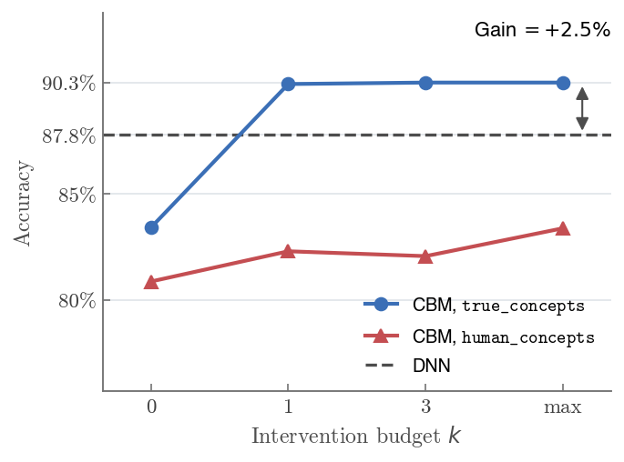
One run, about ten minutes on a laptop. Over the 10 seeds of the paper the CBM reaches 84.5% (true concepts) and 77.6% (human concepts) before interventions, 92.0% and 85.7% after, and the DNN 88.0%.
Sudoku Validation
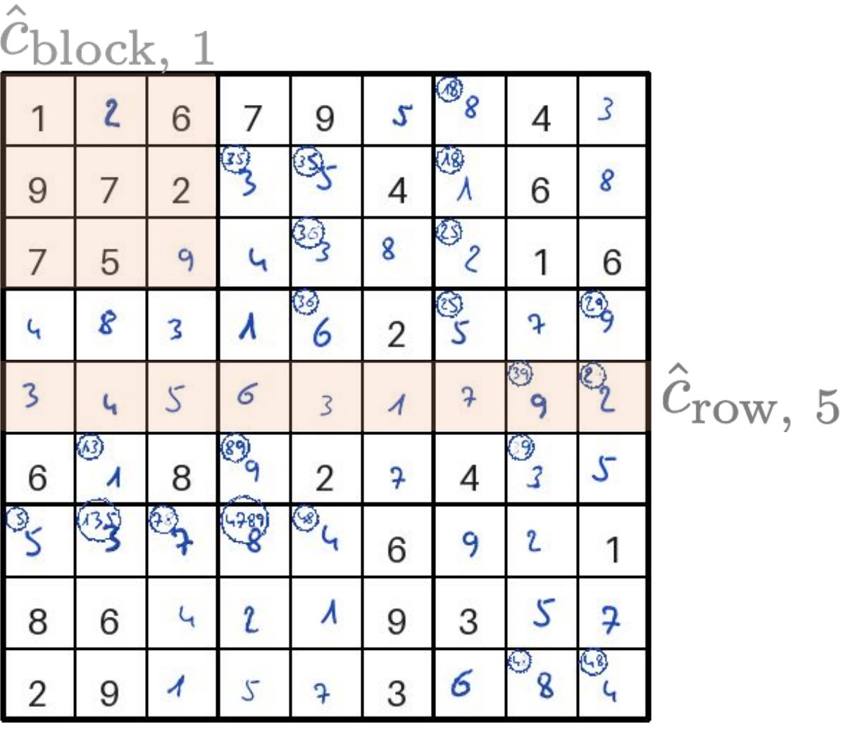
The task is to decide whether a 9×9 board is valid, i.e., contains the digits 1–9 exactly once in each row, column and block. The 27 concepts are the validity of each row, column and block. When the model abstains, a human checks concepts ("is row 5 valid?") until the board is settled or the budget is spent.
Parameters
from concept_benchmark.sudoku import DatasetGenerator

dataset = DatasetGenerator(
    seed=171,                  # random seed
    data_type="image",         # "image" (renders board PNGs) or "tabular" (digit vectors)
    render_images=True,        # set False to skip rendering PNGs (faster, image only)
    block_size=3,              # block size (3 = standard 9×9 board)
    n_boards=1000,             # number of boards to generate
    max_cell_swaps=9,          # corruptions applied to each invalid board, 1 to 9 (each swaps or duplicates digits)
    valid_board_ratio=0.5,     # fraction of valid boards
    # ── Rendering (image only) ──
    font_style="handwritten",  # "handwritten" or "printed"
    font_size=25,              # printed-digit font size at 50 px per cell; every size is this board scaled
    cell_px=50,                # cell size in pixels
    cell_margin_px=2,          # cell margin in pixels
    gridline_px=2,             # grid line width in pixels
    block_border_px=5,         # block border width in pixels
).generate()
Inspecting the data
df = dataset.train.to_dataframe()
show_cols = list(dataset.train.concepts[:5]) + ["label"]
print(df[show_cols])
#      row_valid_1  row_valid_2  row_valid_3  row_valid_4  row_valid_5  label
# 0              1            1            1            1            1      1
# ..           ...          ...          ...          ...          ...    ...
# 301            1            0            0            1            1      0
Pipeline
python scripts/sudoku_pipeline.py --seed 171
python scripts/sudoku_pipeline.py --seed 171 --cbm-family cem

# Harder concept detection: 10 pixels per cell instead of 50
python scripts/sudoku_pipeline.py --seed 171 --cell-px 10

# Save each model's confidence for plot_confidence (optional stage)
python scripts/sudoku_pipeline.py --seed 171 --stages cs intervene selective diagnose plot
| Option | Description |
|---|---|
--cbm-family |
cbm, cem, probcbm or ecbm |
--cell-px |
Pixels per cell (50 by default; at 10 the recognizer misreads a digit on half the boards) |
--target-accuracy |
Selective accuracy that kept predictions must reach (0.90 by default; the paper uses 0.95) |
--stages |
setup ocr cs dnn intervene selective align collect plot, plus the optional diagnose |
Run python scripts/sudoku_pipeline.py --help for the full list of options (including training, intervention, and evaluation parameters).
Training and evaluation
Quickstart: one command trains the paper's models on the handwritten boards of one seed (10 px per cell, where the recognizer misreads a digit on half the boards) and draws the figure below:
python scripts/sudoku_pipeline.py --seed 171 --cell-px 10 --target-accuracy 0.95 --stages setup ocr cs dnn intervene selective collect plot
The same in code, on the digits of each board instead of its image (requires cloning the repo); the blocks are the ones the pipeline is built from:
from concept_benchmark.sudoku import DatasetGenerator
from concept_benchmark.evaluation import plot_automation
from experiments.evaluate import automation_table, coverage_at_target, train_cbm, train_dnn
from experiments.models import GroupPoolingConceptSudokuCNN, SudokuValidatorCNN

dataset = DatasetGenerator(
    seed=171, n_boards=1000, max_cell_swaps=9, data_type="tabular",  # the digits of each board, not its image
).generate_splits()

# CBM: board -> 27 validity concepts -> valid; DNN: board -> valid
cbm = train_cbm(dataset.train, dataset.val, detector=GroupPoolingConceptSudokuCNN,
                epochs=100, patience=20, seed=171, should_propagate=True)
dnn = train_dnn(SudokuValidatorCNN, dataset.train, dataset.val, seed=171)

# both abstain until they are right on 95% of the boards they keep; a human checks up to k concepts of a board the CBM would defer
results = automation_table(cbm, dataset.val, dataset.test, budgets=(1, 3, "max"), target_accuracy=0.95, seed=171)
_, dnn_coverage = coverage_at_target(dnn, dataset.val, dataset.test, target_accuracy=0.95)
print(results[["budget", "coverage_after", "total_concept_checks"]], f"\nDNN coverage: {dnn_coverage:.3f}")

fig, ax = plot_automation(results, n_instances=dataset.test.n, n_concepts=27,
                          baseline_coverage=dnn_coverage, target_accuracy=0.95)
fig.savefig("sudoku_example.png", dpi=150, bbox_inches="tight")
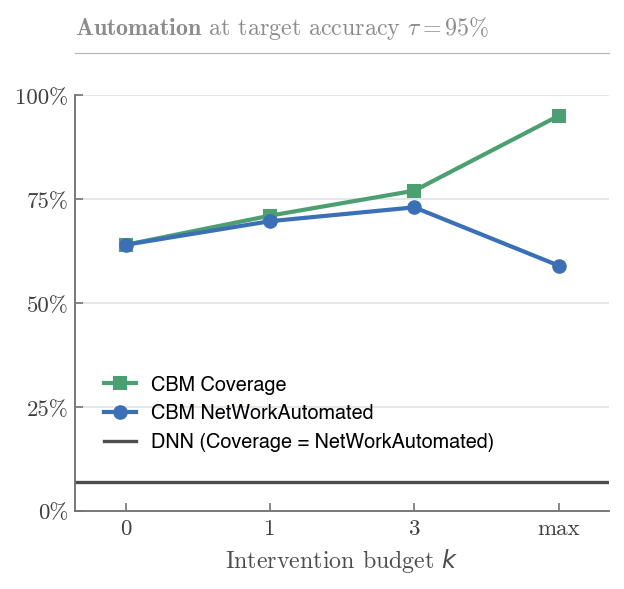
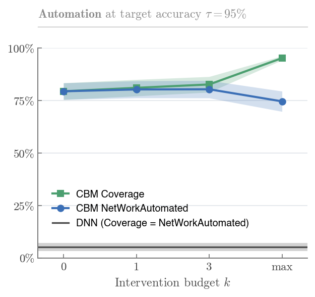
One run of the command above. At 10 px per cell the recognizer misreads a digit on about half the boards, so the CBM answers 64% of the boards on its own (the DNN 7%). Checking up to 3 concepts on the deferred boards raises the boards answered to 77% and the net work automated to 73%; checking all 27 answers 95% of the boards but costs more work than it recovers, and the net work automated falls to 59%. The code block runs on the digits rather than the images, so detection is perfect there and the CBM answers every board.
Benchmark Your Own Model
This guide shows how to evaluate your own concept bottleneck model on the benchmarks provided by this package. All examples below use the robot benchmark, but the same approach works for sudoku.
Prerequisite: You need the full repository (not just
pip install concept-benchmark) to run the pipeline scripts and examples.
Getting data for your model
Generate a dataset as shown in the Quick Start, then access the splits:
train, val, test = dataset.train, dataset.val, dataset.test
Each split is a ConceptDatasetSample with these attributes:
| Attribute | Type | Description |
|---|---|---|
X |
np.ndarray |
Input features (images or tabular) |
C |
np.ndarray |
Concept labels (N, n_concepts) |
y |
np.ndarray |
Target labels (N,) |
concepts |
list[str] |
Concept names |
n_concepts |
int |
Number of concepts |
classes |
list[str] |
Class names |
n |
int |
Number of samples |
Access formats:
# NumPy arrays; X (also .inputs) holds the image file names, the texts or the feature rows
X_train, C_train, y_train = train.X, train.C, train.y

# PyTorch DataLoader
loader = train.loader(batch_size=64, shuffle=True)
for x_batch, c_batch, y_batch in loader:
    ...

# Pandas DataFrame
df = train.to_dataframe()
Splitting
sample() splits the dataset into train/val/test. Sizes can be absolute counts or fractions:
# Absolute counts
dataset.sample(test_size=10000, val_size=1000, train_size=3800, seed=42)

# Fractions (of total dataset size)
dataset.sample(test_size=0.2, val_size=0.2, seed=42)

# Stratified — preserves class proportions in each split
dataset.sample(test_size=0.2, val_size=0.2, stratify=dataset.y, seed=42)

# Group-based — no group appears in multiple splits (group_ids: one id per row, e.g. the robot's identity)
dataset.sample(test_size=0.2, val_size=0.2, groups=group_ids, seed=42)

# Skewed training set — ensure min-fraction of specific concept patterns
dataset.sample(
    test_size=10000, val_size=0.2, train_size=3800,
    sampling_constraints=[{"concepts": {"my_concept": 1}, "min_fraction": 0.3}],
    seed=42,
)
The paper's robot split (generate_splits()) requires a minimum share of each training foot subtype this way; the constraints name subtypes that the preset drops, so split first:
from concept_benchmark.config import PRESET_EXCLUDED_CONCEPTS

dataset = DatasetGenerator(seed=1014, concept_preset="foot_subtypes").generate()
dataset.sample(
    test_size=10000, val_size=0.2, train_size=3800, seed=1014,
    sampling_constraints=[
        {"concepts": {"foot_shape_pointy_4sided": 1}, "min_fraction": 0.30},
    ],
)
# split first: the constraints name subtypes that the preset drops
dataset.drop_concepts(PRESET_EXCLUDED_CONCEPTS["foot_subtypes"])
You can re-split at any time by calling sample() again.
Concept missingness
Simulate missing concept annotations (e.g., incomplete labels from crowdsourcing). Use the generator transforms to produce a new dataset with missingness applied:
from concept_benchmark.transforms import ConceptMissingnessGenerator

dataset.sample(test_size=0.2, val_size=0.2, seed=42)

# MCAR: each concept label independently missing with probability p
dataset = ConceptMissingnessGenerator(dataset, p=0.2, mechanism="mcar", seed=99).generate()

# MNAR: missingness depends on concept value (present concepts more likely observed)
dataset = ConceptMissingnessGenerator(
    dataset, p=0.2, mechanism="mnar", seed=99,
    mnar_config={"present_prob": 0.8, "absent_prob": 0.1},
).generate()
Similarly, ConceptNoiseGenerator adds symmetric or asymmetric label flips, and LabelNoiseGenerator corrupts target labels:
from concept_benchmark.transforms import ConceptNoiseGenerator, LabelNoiseGenerator

dataset = ConceptNoiseGenerator(dataset, p=0.1, seed=99).generate()
dataset = LabelNoiseGenerator(dataset, p=0.05, seed=99).generate()
Wrapping your concept detector
The intervention runner requires a ConceptDetector subclass. Wrap your model:
from experiments.models import ConceptDetector

class MyConceptDetector(ConceptDetector):
    def __init__(self, my_model):
        super().__init__()
        self._my_model = my_model

    def predict_proba(self, dataset, **kwargs):
        """Must return (N, n_concepts) float array in [0, 1]."""
        return self._my_model.predict_concept_probs(dataset.X)
Key point: Override predict_proba() — it receives a ConceptDatasetSample, not raw arrays. Access inputs via dataset.X. The base class predict() calls predict_proba() and thresholds at 0.5 automatically.
Using a PyTorch module directly
If your model is already a PyTorch nn.Module, you can pass it directly instead of subclassing. Your module's forward() must:
- Accept a batched input tensor (e.g.
(B, 3, 32, 32)for images) - Return
(B, n_concepts)raw logits (pre-sigmoid) — sigmoid is applied internally bypredict()
The return value can also be a tuple (first element is used) or a dict with a "logits" key.
cd = ConceptDetector(model=my_pytorch_module)
cd.fit(train, val, fit_params={"epochs": 50, "lr": 1e-3})
You can also split your model into a backbone + concept head using the embedding_model parameter. The detector will probe the backbone's output shape and attach an MLP head automatically:
cd = ConceptDetector(embedding_model=my_backbone)
cd.fit(train, val, fit_params={"epochs": 50, "lr": 1e-3})
Wrapping your label predictor
Subclass FrontEndModel and override predict() and predict_proba():
from experiments.models import FrontEndModel

class MyFrontEnd(FrontEndModel):
    def __init__(self, my_classifier):
        super().__init__()
        self._clf = my_classifier

    def predict(self, C):
        """C is (N, n_concepts) binary 0/1. Returns (N,) int labels."""
        return self._clf.predict(C)

    def predict_proba(self, C):
        """C is (N, n_concepts) binary 0/1. Returns (N, n_classes) probs."""
        return self._clf.predict_proba(C)
Key point: C is already binarized at 0.5 — binary 0/1 values, not probabilities.
For a simple logistic regression baseline, the built-in FrontEndModel() works out of the box:
fe = FrontEndModel()
fe.fit(train.C, train.y)
Assembling and evaluating
Combine your concept detector and label predictor into a ConceptBasedModel:
import numpy as np
from experiments.models import ConceptBasedModel

cbm = ConceptBasedModel(
    concept_detector=MyConceptDetector(my_concept_model),
    label_predictor=MyFrontEnd(my_classifier),
)

predictions = cbm.predict(test)
accuracy = np.mean(predictions == test.y)
print(f"CBM accuracy: {accuracy:.4f}")
For running interventions and alignment on your model, see the Interventions and Alignment section and examples/robot_pipeline_example.py.
Metrics and Plots
concept_benchmark.evaluation has the metrics (accuracy, gain, selective_accuracy, coverage, abstention_threshold, net_work_automated, …) and the plots (plot_intervention_curve, plot_automation, plot_concept_report, …); experiments.evaluate has the blocks that need a model (train_cbm, intervention_table, automation_table, …). The plots take the results tables the pipelines write, average over seeds and draw a standard-error band:
from pathlib import Path
import pandas as pd
from concept_benchmark.evaluation import plot_intervention_curve

# the paper's results: paper-results.zip from the v0.4.0 release; the CBM corrected with the true values
files = Path("paper-results/robot/balanced_rule").glob("*__arch-cbm__isrc-perfect__*__results.csv")
results = pd.concat(pd.read_csv(f) for f in files)
results = results[results["concept_source"].isin(["ground_truth", "human_concepts"])]  # true and human concepts
fig, ax = plot_intervention_curve(results, group="concept_source", baseline_accuracy=0.88)
Metrics and plots reference
Metrics:
| Function | Description |
|---|---|
accuracy(y_pred, y_true) |
Fraction of correct predictions |
delta_accuracy(y_after, y_before, y_true) |
Improvement in accuracy from interventions |
gain(y_pred, y_true, baseline_accuracy) |
Accuracy gain over a baseline model (e.g. DNN) |
selective_accuracy(y_pred, y_true, confidence, threshold) |
Accuracy on non-abstained samples |
coverage(confidence, threshold) |
Fraction of samples where the model does not abstain |
PlattScaling().fit(prob_positive, y_true) |
Calibrates a label probability on validation predictions, as the abstention rule requires |
abstention_threshold(y_true, prob_positive, target_accuracy) |
The paper's abstention rule: the threshold at which the kept predictions reach a target accuracy, and their coverage; fit it on validation predictions |
selective_at(y_true, prob_positive, abstention_threshold, 0.5) |
Selective accuracy and coverage under that threshold |
intervention_metrics(mask, concepts_before, concepts_after, y_prob_before, y_prob_after, y_true, accuracy_before) |
What an intervention did: accuracy, gain, predictions and concepts touched |
net_work_automated(confidence, threshold, n_interventions, n_concepts) |
Net fraction of work automated after intervention cost |
Blocks that need a model live in experiments.evaluate (requires cloning the repo); the pipelines are built from them:
| Function | Returns |
|---|---|
train_cbm(train, validation, seed=..., detector=...) |
The paper's CBM: concept detector plus logistic label predictor |
train_dnn(model, train, validation, seed=...) |
A binary classifier trained with early stopping |
intervention_table(cbm, test, budgets=(1, 3, "max"), seed=...) |
Accuracy at each budget of corrected concepts (the decision-support table) |
automation_table(cbm, validation, test, budgets=(1, 3, "max"), target_accuracy=0.95, seed=171) |
Coverage and checks at each budget under the paper's abstention protocol, label probability calibrated on validation (the automation table) |
coverage_at_target(model, validation, test, target_accuracy) |
Selective accuracy and coverage of any model at a target |
predict_labels(model, dataset), predict_proba_positive(model, dataset) |
Predictions of a DNN or a CBM |
Plots take the results tables that the pipelines write (or your own, with the same columns). Rows from several runs are averaged and drawn with a standard-error band, so pass the concatenated results of all your seeds.
Outcome plots show what happens:
| Function | Shows |
|---|---|
plot_intervention_curve(results, group=..., baseline_accuracy=...) |
The paper's decision-support panel: accuracy against the intervention budget k, one line per model or concept set, with the DNN as a dashed line |
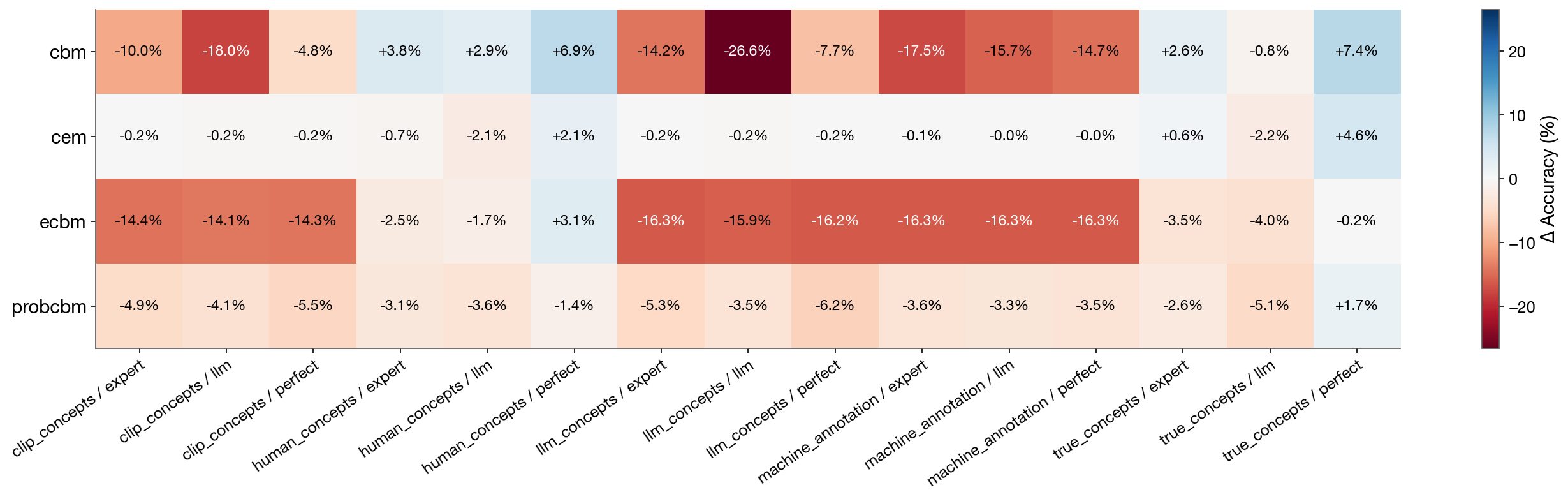
plot_intervention_heatmap(results) |
Change in accuracy from interventions for each model, concept set and intervention source |
plot_alignment_comparison(results) |
Constrained against unconstrained model, before and after interventions |
plot_automation(results, n_instances, n_concepts, baseline_coverage=..., target_accuracy=...) |
The paper's automation panel: Coverage and NetWorkAutomated against the intervention budget, with the DNN's coverage and the target in the title |
plot_selective_classification(dnn_metrics, cbm_metrics) |
DNN against CBM on selective accuracy and coverage |
plot_concept_discovery(ideal_df, subconcept_df, dnn_accuracy) |
True against human concepts at each budget |
plot_model_comparison(results, dnn_accuracy) |
Models × concept sets at each budget |
Diagnostic plots show why:
| Function | Shows | Read it as |
|---|---|---|
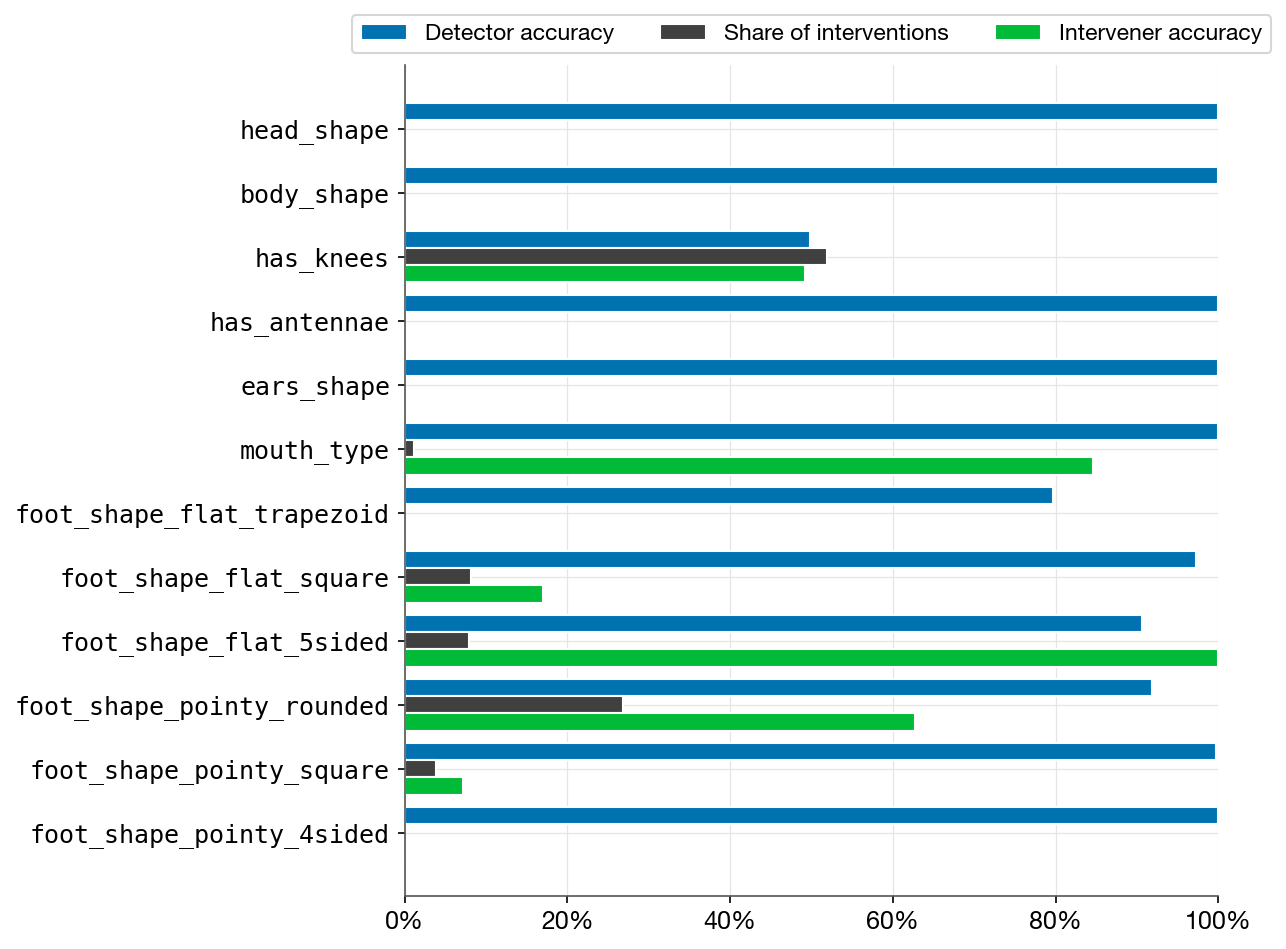
plot_concept_report(mask, concept_proba, concept_answers, concepts_true, concept_names) |
Per concept: detector accuracy, share of interventions, intervener accuracy | An intervener helps only if it is accurate on the concepts the model asks about |
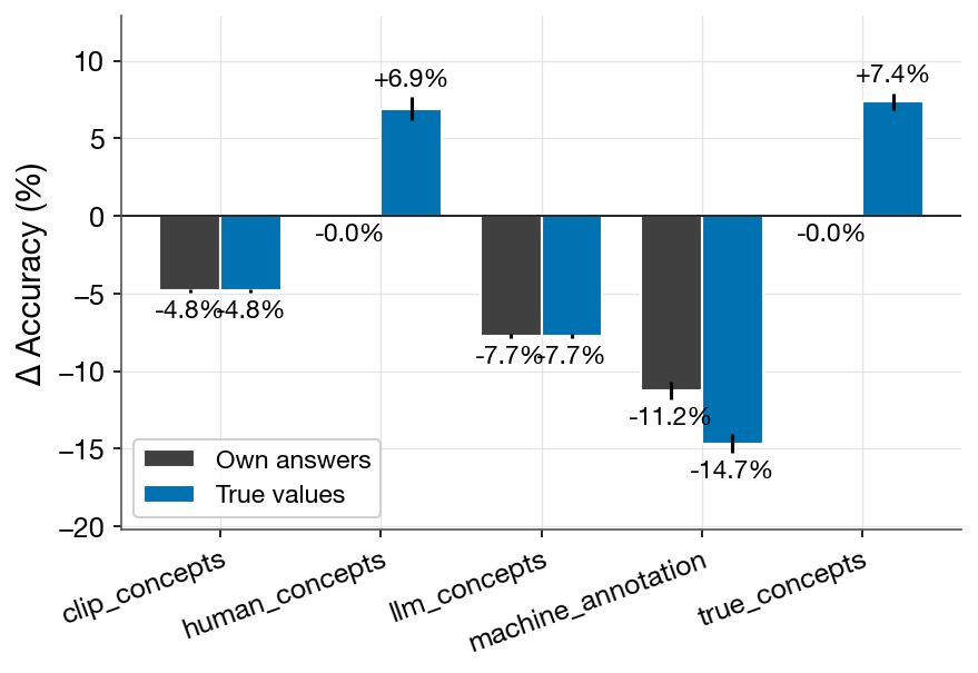
plot_answer_reliance(results) |
Change in accuracy when interventions supply the model's own answers against the true values | Similar bars mean the model does not rely on its concept values |
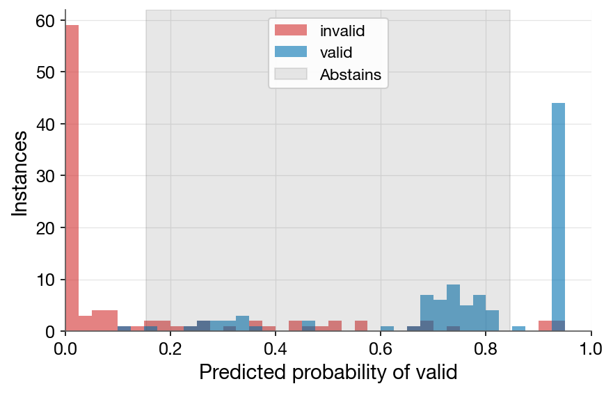
plot_confidence(prob_positive, y_true, abstention_threshold) |
Predicted probabilities by class, with the band where the model abstains | Instances inside the band are deferred no matter how many concepts are checked |
All plot functions return (fig, ax). The pipelines' plot stage draws the ones that apply to a run. The figures below use the 10-seed results of the paper (scripts/paper/make_readme_figures.py).
Interventions and Alignment
Interventions
Interventions are the core benefit of concept bottleneck models: at test time, a user (or automated system) can inspect and correct the model's concept predictions before the final label is determined.
Oracle interventions (manual approach)
The simplest way to run interventions is to directly manipulate concept predictions. After training a ConceptDetector and FrontEndModel, the workflow is:
- Get concept probabilities from the detector
- Identify the most uncertain concepts per sample
- Replace them with ground-truth values
- Re-predict with the label model
import numpy as np
from experiments.models import ConceptDetector, FrontEndModel

# cd and fe are a trained concept detector and label predictor, e.g. cbm.concept_detector and
# cbm.label_predictor of a CBM from experiments.evaluate.train_cbm

# Step 1: Get concept probabilities
concept_probs = cd.predict_proba(test)

# Step 2-3: For each sample, replace the k most uncertain concepts
# with ground-truth values
for k in [1, 3]:
    C_intervened = concept_probs.copy()
    uncertainty = np.abs(concept_probs - 0.5)  # distance from decision boundary
    for i in range(len(test)):
        most_uncertain = np.argsort(uncertainty[i])[:k]
        C_intervened[i, most_uncertain] = test.C[i, most_uncertain]

    # Step 4: Threshold to binary and predict
    preds = fe.predict((C_intervened > 0.5).astype(np.float32))
    acc = np.mean(preds == test.y)
    print(f"k={k}: accuracy={acc:.4f}")
Using the intervention API
For more complex intervention scenarios (budgets, strategies, batched evaluation), use the ConceptInterventionRunner:
import numpy as np
from experiments.models import ConceptBasedModel
from experiments.intervention import ConceptInterventionRunner, InterventionConfig
from experiments.kflip import KFlipInterventionStrategy

# Combine detector and label predictor into a CBM
cbm = ConceptBasedModel(concept_detector=cd, label_predictor=fe)

# Configure the intervention
config = InterventionConfig(
    per_instance_budget=3,  # correct up to 3 concepts per sample
    score_threshold=0.2,          # intervene when the label would change
                                  # with probability 0.2 or more
)

# Run interventions
runner = ConceptInterventionRunner(model=cbm)
strategy = KFlipInterventionStrategy()
result = runner.run(strategy, config, test)

# InterventionResult contains y_prob_before/after and y_pred_after
acc_before = np.mean(np.argmax(result.y_prob_before, axis=1) == test.y)
acc_after = np.mean(result.y_pred_after == test.y)
print(f"Accuracy before: {acc_before:.4f}")
print(f"Accuracy after:  {acc_after:.4f}")
print(f"Concepts corrected: {result.mask.sum()}")
Key classes
InterventionConfig— controls intervention budgets, thresholds, and per-instance capsKFlipInterventionStrategy— the default strategy: evaluates all subsets of up to k concepts per sample and selects the intervention that maximizes predicted confidenceConceptInterventionRunner— coordinates intervention execution and before/after evaluation
Writing a custom strategy
Subclass InterventionStrategy and implement propose(model, batch, config), which returns a StrategyProposal with a boolean mask of the concepts to replace by their true values; prepare() is an optional step run once on the validation set.
Fields, minimal example and the prepare() step
The intervention flow
When ConceptInterventionRunner.run() is called, it:
- Builds an
InterventionBatchfrom the dataset (concept predictions + ground truth) - Calls
strategy.propose(model, batch, config)→ returns aStrategyProposal - Applies the proposal's
maskto replace predicted concepts with ground truth - Re-predicts labels with the corrected concepts
- Returns an
InterventionResultwith before/after predictions
Key data classes
InterventionBatch — the input your strategy receives:
| Field | Type | Description |
|---|---|---|
C_pred |
(N, C) float |
Predicted concept probabilities |
C_true |
(N, C) float |
Ground-truth concept values |
y_true |
(N,) int or None |
True labels (optional) |
n_samples |
int |
Number of samples |
n_concepts |
int |
Number of concepts |
StrategyProposal — what your strategy returns:
| Field | Type | Description |
|---|---|---|
mask |
(N, C) bool |
True = replace prediction with ground truth |
ordering_used |
array or None |
Concept order applied (optional) |
selected_instances |
array or None |
Instance indices that received interventions |
details |
dict |
Additional metadata |
Minimal example
Here's a strategy that intervenes on concepts closest to the 0.5 decision boundary:
import numpy as np
from experiments.intervention import InterventionStrategy, StrategyProposal

class UncertaintyStrategy(InterventionStrategy):
    def __init__(self):
        super().__init__(name="uncertainty")

    def propose(self, model, batch, config):
        k = int(min(config.per_instance_limit(batch.n_concepts), batch.n_concepts))
        mask = np.zeros((batch.n_samples, batch.n_concepts), dtype=bool)

        # Rank concepts by uncertainty (closeness to 0.5)
        uncertainty = 0.5 - np.abs(batch.C_pred - 0.5)
        for i in range(batch.n_samples):
            top_k = np.argsort(uncertainty[i])[-k:]
            mask[i, top_k] = True

        return StrategyProposal(mask=mask)
Use it with the runner:
result = runner.run(
    strategy=UncertaintyStrategy(),
    config=InterventionConfig(per_instance_budget=3, score_threshold=0.2),
    dataset=test,
)
The prepare() step
Override prepare() if your strategy needs a pass over the validation set before inference, for example to precompute a global concept ordering:
class MyStrategy(InterventionStrategy):
    def __init__(self):
        super().__init__(name="my_strategy")

    def prepare(self, model, batch, config):
        """Called once on the validation set before run()."""
        # Compute concept importance from validation data
        self._state["concept_order"] = compute_importance(model, batch)

    def propose(self, model, batch, config):
        order = self._state["concept_order"]
        # ... use precomputed order
Call runner.prepare() before runner.run() to run it:
runner.prepare(strategy, config, validation_dataset=val)
result = runner.run(strategy, config, dataset=test)
Concept sources and intervention sources
The robot pipeline varies two things independently: who annotates the concepts a model is trained on, and who answers when the model asks about a concept at test time.
| Concept source | Concepts |
|---|---|
| ground_truth | The 7 true concepts |
| human_concepts | 12 concepts as a human annotator would list them (six foot subtypes) |
| noisy_human_concepts | The same concepts, annotated with 20% label noise (annotators who disagree) |
| machine_annotation | The human concepts, scored by CLIP (label-free CBM) |
| llm_concepts | Concepts written by an LLM, scored by CLIP |
| clip_concepts | Single words chosen by CLIP, scored by CLIP |
| Intervention source | Answers |
|---|---|
| perfect | The true concept values — the upper bound |
| expert | A simulated expert, correct 80% of the time on every concept |
| llm | An LLM that answers each concept from the image (Gemini by default) |
| self | The model's own thresholded predictions — changes no value, so it isolates the effect of the intervention mechanism |
python scripts/robot_pipeline.py --seed 1014 --concept-preset foot_subtypes \
    --concept-sources human_concepts machine_annotation \
    --intervention-sources perfect expert self --budgets 1 3 max
LLM interventions need an API key (--llm-api-key or GEMINI_API_KEY); --llm-cache-only reuses saved answers.
Regimes
--regimes names the pairings of the first version of the benchmark: baseline (human concepts, corrected with the true values), expert (corrected by an 80%-accurate expert), subjective (concepts with 20% label noise, expert), machine (CLIP-scored concepts, expert), llm and clip (LLM-written or CLIP-chosen concepts, corrected by an LLM).
python scripts/robot_pipeline.py --seed 1014 --concept-preset foot_subtypes --regimes baseline expert subjective
python scripts/robot_text_pipeline.py --seed 1337 --regimes baseline expert subjective
For a complete end-to-end example with training, interventions (through the intervention_table block, which runs ConceptInterventionRunner with the paper's policy) and alignment, see examples/robot_pipeline_example.py.
Alignment
Alignment constraints force the label predictor's concept weights to match a user's prior expectations about concept-label relationships. For example, if a domain expert knows that "has knees" should positively predict the Glorp class, alignment constrains that weight to be positive during retraining.
Why alignment matters
In standard CBM training, the label predictor (logistic regression on concept activations) learns weights freely from data. This can produce counterintuitive weights — e.g., has_knees getting a negative weight even when knees truly indicate Glorp — because the model exploits correlations among imperfect concept predictions.
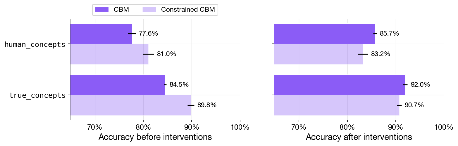
The paper shows that an alignment constraint can:
- Raise accuracy before interventions — the constrained model no longer relies on a concept its detector reads at chance.
- Remove the benefit of interventions — after every concept is corrected, the unconstrained model is the more accurate one.
The constraint closes the pathway through which a corrected concept reaches the label.
Usage
After training a ConceptBasedModel, use run_alignment() to retrain the frontend with sign constraints and compare:
from experiments.utils import run_alignment

results = run_alignment(
    concept_based_model=cbm,
    train_dataset=train,
    test_dataset=test,
    monotonicity_constraints={"has_knees": 1},  # require a non-negative weight
)

print(f"Original accuracy: {results['original_accuracy']:.4f}")
print(f"Aligned accuracy:  {results['aligned_accuracy']:.4f}")
print(f"Accuracy change:   {results['accuracy_change']:+.4f}")
The monotonicity_constraints dict maps concept names to their required sign: +1 for positive weight, -1 for negative.
Expected results
Mean accuracy over the 10 seeds of the paper (balanced rule):
| Concepts | CBM (k=0) | Constrained (k=0) | CBM (k=max) | Constrained (k=max) |
|---|---|---|---|---|
| true (7 concepts) | 84.5% | 89.8% | 92.0% | 90.7% |
| human (12 concepts) | 77.6% | 81.0% | 85.7% | 83.2% |
For a complete end-to-end example with training, interventions, and alignment, see examples/robot_pipeline_example.py.
Reproducing the Paper
EXPERIMENTS.md lists the commands behind each experiment, and scripts/paper/README.md maps every table, figure and test of the paper to the script that produces it.
The paper's results (paper-results.zip, 14 MB) are attached to the v0.4.0 release; unpack them and pass the folder to any paper script as --results-root.
Citation
If you use this package in your research, please cite:
@inproceedings{skirzynski2026measuring,
  title={Measuring What Matters: Synthetic Benchmarks for Concept Bottleneck Models},
  author={Skirzy{\'n}ski, Julian and Cheon, Harry and Kadekodi, Shreyas and Stewart, Meredith and Ustun, Berk},
  booktitle={Advances in Neural Information Processing Systems},
  year={2026},
}
1 maintainer

Metadata
1 maintainer
Release files for concept-benchmark 0.4.1
For a detailed explanation of source distributions (sdists) and built distributions (wheels), please see the package formats documentation.
Source distribution (sdist)
| File | Size | Uploaded | |
|---|---|---|---|
| concept_benchmark-0.4.1.tar.gz | 3.2 MB | Details |
Built distribution (wheel)
| File | Interpreter | ABI | Platform | Reset |
|---|---|---|---|---|
| concept_benchmark-0.4.1-py3-none-any.whl | Python 3 | none | any | Details |
Total release size: 3.9 MB
Release files / concept_benchmark-0.4.1.tar.gz
| Download URL | concept_benchmark-0.4.1.tar.gz |
|---|---|
| Size | 3.2 MB |
| Tags | Source |
|
SHA-256 checksum How to use checksums |
733f6bcc500e33799fa81db08735e588112f7d1ad5939670f557a56620f87d1d
|
|
BLAKE2b-256 checksum How to use checksums |
411b40d584d5a29a276c43b18e65d2a22dba2292bddf4692d68140ee345319ba
|
| Upload date | |
|
Uploaded using Trusted Publishing? What is trusted publishing? |
No |
| Uploaded via |
uv/0.10.9 {"installer":{"name":"uv","version":"0.10.9","subcommand":["publish"]},"python":null,"implementation":{"name":null,"version":null},"distro":{"name":"macOS","version":null,"id":null,"libc":null},"system":{"name":null,"release":null},"cpu":null,"openssl_version":null,"setuptools_version":null,"rustc_version":null,"ci":null}
|
Release files / concept_benchmark-0.4.1-py3-none-any.whl
| Download URL | concept_benchmark-0.4.1-py3-none-any.whl |
|---|---|
| Size | 678.5 kB |
| Tags | Python 3 |
|
SHA-256 checksum How to use checksums |
5f0d2bdc813fe27669f94ceedbe3da57b62ca367de9a411d534086788053de49
|
|
BLAKE2b-256 checksum How to use checksums |
e79fef5038150db6ec151bc2120e40afb55990ec2a430ed2481e119338c7d065
|
| Upload date | |
|
Uploaded using Trusted Publishing? What is trusted publishing? |
No |
| Uploaded via |
uv/0.10.9 {"installer":{"name":"uv","version":"0.10.9","subcommand":["publish"]},"python":null,"implementation":{"name":null,"version":null},"distro":{"name":"macOS","version":null,"id":null,"libc":null},"system":{"name":null,"release":null},"cpu":null,"openssl_version":null,"setuptools_version":null,"rustc_version":null,"ci":null}
|














