
CongestGym
A Gymnasium environment for reinforcement learning on congested packet networks:
allocate bandwidth and choose routes, together.




When a network is congested, an operator has two levers: how much bandwidth
each link gets and which paths traffic takes. The two interact, yet open
reinforcement-learning (RL) environments for networking either control routing
alone or need a full ns-3 installation. CongestGym gives an agent both levers at
once, in a lightweight pure-Python packet simulator that installs with pip
and runs on a laptop.
Every step the agent sets a bandwidth weight and a routing weight for each link, under a total bandwidth budget, and is rewarded for delivered traffic minus delay, packet loss and missed deadlines across four traffic classes (voice, gaming, video, best effort).
What ships with it
- A store-and-forward packet simulator with finite buffers, per-link queues, shortest-path routing with random equal-cost multipath, and node bottlenecks.
- Grid, ring, star, mesh and random topologies, plus the real Abilene research backbone with one week of measured traffic (SNDlib).
- Single-agent Gymnasium and multi-agent PettingZoo interfaces.
- Six rule-based baselines and a fluid multi-commodity-flow upper bound.
- Scripts to train PPO / SAC / TD3 (Stable-Baselines3), evaluate on held-out seeds, benchmark, and animate two policies side by side.
- A reproducible evaluation protocol (separate training, validation and test seeds; choices fixed in advance) and the committed results of the study below.
Main finding. PPO delivers more traffic than every rule-based policy in two of the four scenarios studied: a grid with one degraded router (by the widest margin) and an irregular random graph. It does not on a symmetric grid, and on the real Abilene backbone a simple congestion-aware rule beats both learned agents. Controlling both levers helps the learner only where both matter. The numbers are under Results.
Contents
Installation · Quick start · Demo · How the environment works · Baselines · Training and evaluation · Results · Datasets · Notebooks · Tests · Limitations · Repository layout · Contributing and citing
Installation
Python 3.10 or newer.
From GitHub, as a package:
pip install "congestgym[rl] @ git+https://github.com/spaciouskarter78/congestgym"
For development, to run the scripts, notebooks and tests:
git clone https://github.com/spaciouskarter78/congestgym.git
cd congestgym
python -m venv .venv
source .venv/bin/activate              # Windows PowerShell: .\.venv\Scripts\Activate.ps1
pip install -e ".[all]"
export PYTHONPATH=.                    # PowerShell: $env:PYTHONPATH = "."
PYTHONPATH=. lets the scripts in examples/, scripts/ and qa/ import the
repository. To use the exact versions the results were produced with, install
with pip install -r requirements.txt -c constraints.txt instead.
| Extra | Adds | Needed for |
|---|---|---|
| (none) | Gymnasium, NumPy, NetworkX, pandas, Matplotlib | the environment and baselines |
rl |
PyTorch, Stable-Baselines3 | training agents, the demo with a trained agent |
marl |
PettingZoo | MultiAgentCongestGymEnv |
bounds |
SciPy | the flow upper bound |
notebooks |
Jupyter | re-running the notebooks |
dev |
pytest | the test suite |
all |
all of the above |
Quick start
import gymnasium as gym
import congestgym                                   # registers CongestGym-v0
from congestgym.baselines import POLICIES

env = gym.make("CongestGym-v0", topology="grid", num_nodes=9,
               bandwidth_budget=0.6, load_scale=1.25)
obs, info = env.reset(seed=2000)

policy = POLICIES["congestion_aware"]               # or use your agent's actions
for _ in range(200):
    action = policy(env.unwrapped, obs)             # E bandwidth weights, then E routing weights
    obs, reward, terminated, truncated, info = env.step(action)
    if terminated or truncated:
        break

print(info["delivered_units"], info["dropped_units"], info["reward_delay"])
Main constructor options: topology (grid, ring, star, mesh,
random, abilene), num_nodes, link_capacity, node_buffer,
load_scale, bandwidth_budget, bottlenecks, traffic, the reward
coefficients k, c, m and delay_reference, max_steps, render_mode
(human or rgb_array), and the simulator options topology_seed,
queueing, tie_break and service_order (see
Simulation model).
Train an agent and compare it with every baseline on held-out seeds:
python examples/train_agent.py --algo ppo --timesteps 500000 --seed 0 --load-scale 1.25 --budget 0.6
Demo
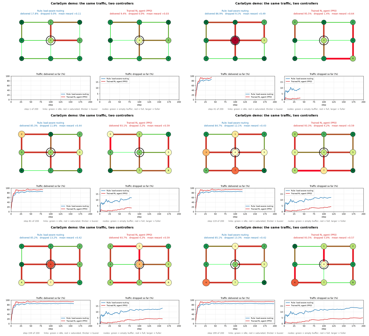
python examples/demo.py                                   # live window
python examples/demo.py --save demo.gif                   # write the animation to a file
python examples/demo.py --left max_bandwidth --right queue_proportional
python examples/demo.py --seed 2005 --bottleneck none     # plain grid, no degraded node
Two controllers receive exactly the same traffic. Links are coloured from
green (idle) to red (saturated), nodes by how full their buffers are, and
the charts track the share of offered traffic each side has delivered and
dropped so far. --left and --right take any baseline name, or ppo /
sac for an agent saved by examples/train_agent.py. By default the demo
runs the degraded-node grid (centre node at half capacity, budget 0.8) with
the PPO agent trained on it (results/rl/grid_bottleneck_b08/ppo_seed0)
against the best rule there, load_aware_routing; --seed values from
2000 upwards are traffic the agent never saw. The percentages cover the whole
episode from step 0, so they differ slightly from the tables below, which
skip a 20-step warm-up.
How the environment works
Simulation model
The environment is a store-and-forward packet simulator, not a flow-rate approximation.
- Nodes hold finite buffers. Packets physically occupy them.
- Links are undirected and have a service rate (units per step) shared by both directions. The bandwidth action scales that rate.
- Packets advance at most one hop per step. Service is fractional: a packet larger than the budget a link has left is partly transmitted and finishes the hop on a later step, so any positive allocation moves traffic.
- Each node keeps one FIFO queue per outgoing link, all sharing the
node's buffer. A packet waiting for an exhausted link blocks only traffic
for that link (
queueing="shared_fifo"restores one FIFO per node, where the head packet blocks every link). - Nodes are served in a fresh random order each step, so no node gets
first use of a shared link because of its id (
service_order="id"). - A packet moves on only if the next node had room at the start of the step
(plus what has arrived since); otherwise it is dropped. Buffers therefore
never exceed
node_buffer. - Routing is decided when a packet is admitted: shortest path under the
per-link routing weights in the current action. Among equal-cost next
hops the packet picks one at random (per-packet ECMP);
tie_break="first"takes the lowest id. Uniform weights give hop-count shortest paths. - Randomness:
seeddrives traffic, tie-breaks and service order; therandomtopology is drawn fromtopology_seed(default 0), so the graph and the action space do not change with the episode seed. - Latency is measured in steps from injection to delivery.
- Loss occurs on admission overflow, downstream buffer overflow, or when no route exists.
Observation and action
E = number of links, N = number of nodes (default grid: E=12, N=9).
| Shape | Meaning | |
|---|---|---|
| Observation | Box(0, 1, (2E+N,)) |
link utilization (E), pending demand per link (E), node buffer occupancy (N) |
| Action | Box(0, 1, (2E,)) |
per-link bandwidth weight (E), then per-link routing weight (E) |
bandwidth_budget=b caps the sum of bandwidth weights at b*E; actions above
it are scaled down proportionally. Without a budget, "allocate everything
everywhere" is close to optimal and the allocation problem is uninteresting.
Reward
R = Throughput - k*Delay - c*PacketLoss - m*DeadlineMiss (defaults k=0.5, c=1.0, m=0.5)
Every term is normalized to [0, 1] per step:
- Throughput: delivered / offered units, clipped at 1.
- Delay: delay-sensitivity-weighted mean age of traffic in the system
(end-to-end delay of packets delivered this step, current age of packets
still queued), divided by
delay_reference(10 steps) and clipped at 1. It is QoS-weighted, not plain latency: voice and gaming cost more per step than best-effort. - PacketLoss: dropped / offered units, clipped at 1.
- DeadlineMiss: packets that missed their class deadline this step (delivered late, or expired while queued) over packets resolved this step. Each packet is counted once.
The reward is therefore in [-2, 1]. info reports every term and the raw
counters. The terms are per-step quantities; for the fraction of traffic
delivered or dropped over an episode, aggregate the raw counters
(congestgym.utils.qos.EpisodeQoS).
Traffic
TrafficGenerator draws Poisson arrivals for four QoS classes with different
packet sizes, delay sensitivities and deadlines (about 104 units per step at
load_scale=1). TraceTrafficGenerator replays a step,src,dst,volume CSV,
rescaled to a target_load (see Datasets). Any object with
generate(step) and reset(seed) can be passed as traffic=.
Seeding: reset(seed=s) replays the same traffic; reset() continues the
random stream, so successive episodes see new traffic.
Node bottlenecks
bottlenecks={node: scale} degrades a node: it keeps only that fraction of
its buffer and of the capacity of every link touching it. A policy then has to
steer traffic around the degraded node or prioritise its links.
Multi-agent
MultiAgentCongestGymEnv exposes the same simulator through the PettingZoo
parallel API. Each link is controlled by exactly one of its endpoint nodes;
nodes that control no link are not agents. Agents share the global
observation and a cooperative reward. step() needs one action for every
live agent and raises otherwise. It needs the marl extra.
Baselines
All in congestgym/baselines.py; each takes (env, obs) and returns an action.
| Policy | Bandwidth | Routing |
|---|---|---|
max_bandwidth |
equal split over all links | hop-count shortest path |
queue_proportional |
proportional to each link's pending demand | hop-count shortest path |
load_aware_routing |
equal split | load-aware shortest path (congested links cost more) |
congestion_aware |
proportional to pending demand | load-aware shortest path |
random |
uniform random | uniform random |
min_bandwidth |
5% everywhere | hop-count shortest path |
load_aware_routing and congestion_aware are the routing-aware
traffic-engineering baselines. Their constants can be changed with
congestgym.baselines.make_policy, e.g.
make_policy("congestion_aware", floor=0.1, base=0.3).
Training and evaluation
| Task | Command |
|---|---|
| Train one agent (PPO, SAC or TD3) | python examples/train_agent.py --algo ppo --timesteps 500000 --seed 0 --load-scale 1.25 --budget 0.6 |
| Train only one half of the action | add --control bandwidth or --control routing |
| Train on Abilene | python examples/train_agent.py --algo ppo --topology abilene --nodes 12 --trace data/abilene_trace_20040301_7d.csv.gz --load 120 --budget 0.8 --trace-random-start |
| All scenarios, 5 seeds each (restartable queue) | python scripts/run_training_matrix.py --workers 10 --ppo-steps 500000 --sac-steps 100000 |
| Reward table and learning curves of a folder | python scripts/summarize_training.py results/rl/<folder> |
| Delivered / dropped / delay of saved agents | python scripts/evaluate_saved.py results/rl/<folder> |
| Fluid upper bound | python scripts/flow_bound.py |
| Baseline scenario matrix | python scripts/run_benchmark.py (or --quick) |
| Refresh the tables in this README | python scripts/update_readme_results.py |
train_agent.py writes train_monitor.csv (training returns),
eval_curve.csv (reward on validation seeds every --eval-every steps),
final_eval.csv (the agent and every baseline on the test seeds) and
model.zip to --out (default results/<algo>_seed<seed>/). Agents act on a
[-1, 1] action space and train on the constrained setting (--budget below
1); without a budget there is little to learn.
Seed protocol. Training environments use seeds from --seed upwards and
then draw fresh traffic every episode; learning curves use validation seeds
(1000+); every reported table uses test seeds 2000 to 2009, which neither
training nor the curves saw. Choices of scenario, hyperparameters and baseline
constants are made on validation seeds only.
Results
Everything in this section is copied from files under results/ by
scripts/update_readme_results.py. Rewards are the mean per-step reward after
a 20-step warm-up, over 200-step episodes. How each scenario was chosen, with
the rules fixed before training, is in docs/HEADLINE_SCENARIO.md and
docs/ABILENE_SCENARIO.md; the full readings are listed in
Documentation.
Learned agents against rule-based policies
PPO and SAC on four scenarios, five training seeds each, plus PPO ablations that control only one half of the action. Training budgets: PPO 500,000 steps, SAC 100,000. Delivered traffic:
Delivered % of offered traffic, test seeds 2000-2009, steps 20..199, mean ± 95% CI (agents: over 5 training seeds; rule-based: over test episodes). The best rule-based policy is picked per row on the test seeds. Ablation rows: PPO controls one half of the action, the rule-based policies both. Flow bound: congestgym/bounds.py, an upper limit that is loose (see docs/RL_RESULTS_0.4.0.md, section 2.6).
| Training folder | Flags | PPO | SAC | Best rule-based policy | Flow bound |
|---|---|---|---|---|---|
grid_l125_b06 |
--load-scale 1.25 --budget 0.6 |
73.5 ± 0.6 | 68.6 ± 1.3 | congestion_aware 74.1 ± 1.4 | 90.3 |
grid_bottleneck_b08 |
--bottleneck 4:0.5 |
94.6 ± 0.3 | 90.3 ± 1.4 | load_aware_routing 85.0 ± 0.8 | 100.0 |
abilene_l120_b08 |
--topology abilene --nodes 12 --trace data/abilene_trace_20040301_7d.csv.gz --load 120 --budget 0.8 --trace-random-start |
75.4 ± 3.3 | 78.5 ± 2.3 | congestion_aware 80.7 ± 8.5 | 92.5 |
random9_l15_b06 |
--topology random --topology-seed 0 --load-scale 1.5 --budget 0.6 |
81.3 ± 0.4 | 76.1 ± 1.8 | queue_proportional 79.7 ± 0.7 | 99.4 |
grid_l125_b06_bandwidth_only |
--load-scale 1.25 --budget 0.6 --control bandwidth |
72.9 ± 0.3 | n/a | congestion_aware 74.1 ± 1.4 | 90.3 |
grid_l125_b06_routing_only |
--load-scale 1.25 --budget 0.6 --control routing |
72.2 ± 0.2 | n/a | congestion_aware 74.1 ± 1.4 | 90.3 |
random9_l15_b06_routing_only |
--topology random --topology-seed 0 --load-scale 1.5 --budget 0.6 --control routing |
66.3 ± 0.2 | n/a | queue_proportional 79.7 ± 0.7 | 99.4 |
grid_bottleneck_b08_bandwidth_only |
--bottleneck 4:0.5 --control bandwidth |
72.8 ± 1.1 | n/a | load_aware_routing 85.0 ± 0.8 | 100.0 |
grid_bottleneck_b08_routing_only |
--bottleneck 4:0.5 --control routing |
93.8 ± 0.2 | n/a | load_aware_routing 85.0 ± 0.8 | 100.0 |
random9_l15_b06_bandwidth_only |
--topology random --topology-seed 0 --load-scale 1.5 --budget 0.6 --control bandwidth |
80.8 ± 0.2 | n/a | queue_proportional 79.7 ± 0.7 | 99.4 |
PPO delivers more than every rule-based policy in two of the four scenarios,
the degraded-node grid (grid_bottleneck_b08, by the widest margin) and the
random graph. It does not on the headline grid, where it delivers about as much
as congestion_aware but with longer delays and more missed deadlines, so its
reward is lower; nor on the real Abilene topology and trace, where
congestion_aware delivers more than both PPO and SAC. Controlling both halves
of the action does not help PPO on the headline compared with bandwidth alone.
Paired statistics, convergence and the ablations are in
docs/RL_RESULTS_0.4.0.md and docs/ABILENE_RESULTS.md.
Headline scenario in detail (3x3 grid, load x1.25, budget 0.6): reward, delivered, dropped, delay
| Policy | Kind | Reward (mean ± 95% CI) | n | CI over |
|---|---|---|---|---|
| congestion_aware | baseline | +0.099 ± 0.025 | 10 | test episodes |
| queue_proportional | baseline | +0.093 ± 0.025 | 10 | test episodes |
| load_aware_routing | baseline | +0.045 ± 0.020 | 10 | test episodes |
| PPO | RL agent | +0.037 ± 0.016 | 5 | training seeds |
| max_bandwidth | baseline | -0.034 ± 0.033 | 10 | test episodes |
| SAC | RL agent | -0.059 ± 0.033 | 5 | training seeds |
| random | baseline | -0.581 ± 0.019 | 10 | test episodes |
| min_bandwidth | baseline | -1.729 ± 0.007 | 10 | test episodes |
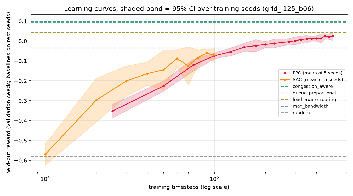
Scenario grid_l125_b06 (--load-scale 1.25 --budget 0.6). Episode aggregates over steps 20..199 of test seeds 2000..2009, mean ± 95% CI (agents: over training seeds; baselines: over test episodes). Delivered % and Dropped % are of traffic offered in the same window; the remainder is backlog growth. The random row draws its own actions here, so its reward differs slightly from the reward table. Agent and deterministic-baseline rewards match final_eval.csv (600 compared, max difference 2.2e-16).
| Policy | Reward | Delivered % | Dropped % | Delay of delivered packets (steps) | Deadline misses per delivered packet |
|---|---|---|---|---|---|
| congestion_aware | +0.099 | 74.1 ± 1.4 | 25.8 ± 1.2 | 5.16 ± 0.09 | 0.330 ± 0.010 |
| queue_proportional | +0.093 | 73.2 ± 1.5 | 26.9 ± 1.4 | 5.03 ± 0.09 | 0.319 ± 0.007 |
| load_aware_routing | +0.045 | 72.5 ± 1.5 | 27.5 ± 1.2 | 5.42 ± 0.06 | 0.349 ± 0.005 |
| PPO | +0.037 | 73.5 ± 0.6 | 26.4 ± 0.5 | 5.82 ± 0.11 | 0.370 ± 0.006 |
| max_bandwidth | -0.034 | 68.5 ± 1.5 | 31.4 ± 1.3 | 5.38 ± 0.09 | 0.358 ± 0.010 |
| SAC | -0.059 | 68.6 ± 1.3 | 31.3 ± 1.2 | 5.82 ± 0.40 | 0.381 ± 0.023 |
| random | -0.581 | 49.4 ± 1.0 | 50.4 ± 0.8 | 7.96 ± 0.22 | 0.602 ± 0.010 |
| min_bandwidth | -1.729 | 5.5 ± 0.3 | 94.5 ± 0.3 | 52.02 ± 2.35 | 2.545 ± 0.050 |
Read "delivered" and "dropped" from these tables, not from the reward terms:
the throughput and loss terms in the reward are ratios within a single
step (and throughput is clipped at 1), so their average over an episode is
not the fraction of traffic delivered.
Upper bound
congestgym/bounds.py (extra bounds) solves a fluid multi-commodity-flow
linear program: the expected traffic matrix, link capacities and the budget,
with the allocation chosen optimally. No policy can exceed it in the long run.
It is loose: it ignores queueing and lets the optimiser drop the
longest-distance traffic first, which no policy here can do. Read the room
below it as an upper limit, not as headroom.
Fluid flow upper bound on the delivered fraction (%), from congestgym/bounds.py: the expected traffic matrix, link capacities and the bandwidth budget, with the allocation chosen optimally. No policy can exceed it in the long run; a finite window can exceed it slightly through backlog carried in. Policy figures: delivered % on test seeds 2000-2009, steps 20..199. The bound is loose (docs/RL_RESULTS_0.4.0.md, section 2.6): the room below it is an upper limit on what any policy could gain, not a measure of it. The trace row's bound uses the trace's mean matrix over the week and ignores its daily cycle, so it is looser still.
| Scenario | Bound, free routing | Bound, shortest paths | Best heuristic | PPO | SAC |
|---|---|---|---|---|---|
| grid_l125_b06 | 90.3 | 90.3 | congestion_aware 74.1 | 73.5 | 68.6 |
| grid_bottleneck_b08 | 100.0 | 100.0 | load_aware_routing 85.0 | 94.6 | 90.3 |
| abilene_l120_b08 | 92.5 | 92.5 | congestion_aware 80.7 | 75.4 | 78.5 |
| random9_l15_b06 | 99.4 | 99.4 | queue_proportional 79.7 | 81.3 | 76.1 |
The bound is the same with free multipath routing and with shortest-path routing in every scenario tested, so the routing action's gains here are dynamic (spreading load as queues change), not extra capacity.
Follow-up experiments (E1 to E4)
Planned in docs/NEXT_EXPERIMENTS.md with every decision rule fixed before
the runs; results in docs/E1_E4_RESULTS.md and docs/E2_E3_RESULTS.md.
- E1, tuned rule-based policies. The heuristics' constants were tuned on
validation seeds. PPO's wins on the degraded-node grid and the random graph
hold against the strongest rule-based policy, tuned or not. On the headline
the published
congestion_awarewas already as good as its tuned versions. (E1 also covered a trace scenario that was later withdrawn; it was not repeated on Abilene.) - E2, tuned PPO on the headline. Eight PPO configurations were compared
on validation seeds; the winner (gamma 0.99, entropy coefficient 0.01) was
recorded before any test result was read, then evaluated once. The
pre-registered outcome: tuning does not close the gap. Tuned PPO is
better than the original on delay and deadline misses but still below
congestion_awareon reward. - E3, ablations on the degraded-node grid and the random graph (rows
*_onlyin the first table). Controlling both halves of the action helps the learner only on the degraded-node grid; on the random graph bandwidth alone is as good, and on the headline neither half adds to the other. - E4, detours. On the degraded-node grid no policy detours more than about 1% of packets; on the random graph the routing heuristics detour far more often than PPO, which almost never does.
E2: tuned PPO on the headline scenario
Scenario g0.99_lr3e-4_ent0.01 (--load-scale 1.25 --budget 0.6 --gamma 0.99 --lr 3e-4 --ent-coef 0.01). Episode aggregates over steps 20..199 of test seeds 2000..2009, mean ± 95% CI (agents: over training seeds; baselines: over test episodes). Delivered % and Dropped % are of traffic offered in the same window; the remainder is backlog growth. The random row draws its own actions here, so its reward differs slightly from the reward table. Agent and deterministic-baseline rewards match final_eval.csv (300 compared, max difference 2.2e-16).
| Policy | Reward | Delivered % | Dropped % | Delay of delivered packets (steps) | Deadline misses per delivered packet |
|---|---|---|---|---|---|
| congestion_aware | +0.099 | 74.1 ± 1.4 | 25.8 ± 1.2 | 5.16 ± 0.09 | 0.330 ± 0.010 |
| queue_proportional | +0.093 | 73.2 ± 1.5 | 26.9 ± 1.4 | 5.03 ± 0.09 | 0.319 ± 0.007 |
| PPO | +0.056 | 73.5 ± 0.7 | 26.4 ± 0.7 | 5.58 ± 0.05 | 0.357 ± 0.004 |
| load_aware_routing | +0.045 | 72.5 ± 1.5 | 27.5 ± 1.2 | 5.42 ± 0.06 | 0.349 ± 0.005 |
| max_bandwidth | -0.034 | 68.5 ± 1.5 | 31.4 ± 1.3 | 5.38 ± 0.09 | 0.358 ± 0.010 |
| random | -0.581 | 49.4 ± 1.0 | 50.4 ± 0.8 | 7.96 ± 0.22 | 0.602 ± 0.010 |
| min_bandwidth | -1.729 | 5.5 ± 0.3 | 94.5 ± 0.3 | 52.02 ± 2.35 | 2.545 ± 0.050 |
Baseline scenario matrix
All six baselines on five topologies, three loads and two budgets, plus the
degraded node and four Abilene settings (python scripts/run_benchmark.py).
In most scenarios the leading heuristics are statistically tied; rows where
every policy is far below zero are overloaded regimes in which no policy can
do well. On Abilene congestion_aware delivers the most in every cell; since
each episode starts at a random point of the week, rewards vary between
episodes, so compare policies on the same seeds.
Reward, all scenarios
Mean post-warmup reward ± 95% CI over 10 seeds (2000..2009), 200 steps, warmup 20.
Bold: best policy, its interval overlaps no other. ~: best group, intervals overlap (a statistical tie).
| Scenario | random | min_bandwidth | max_bandwidth | queue_proportional | load_aware_routing | congestion_aware |
|---|---|---|---|---|---|---|
| grid/load x0.5/budget 0.8 | +0.430 ± 0.031 | -1.465 ± 0.023 | +0.723 ± 0.007 | +0.613 ± 0.013 | +0.696 ± 0.008 | +0.590 ± 0.006 |
| grid/load x0.5/budget 0.5 | +0.394 ± 0.029 | -1.465 ± 0.023 | +0.625 ± 0.011 ~ | +0.605 ± 0.012 ~ | +0.618 ± 0.010 ~ | +0.576 ± 0.008 |
| grid/load x1/budget 0.8 | -0.268 ± 0.046 | -1.688 ± 0.008 | +0.629 ± 0.012 | +0.593 ± 0.008 | +0.666 ± 0.008 | +0.590 ± 0.011 |
| grid/load x1/budget 0.5 | -0.377 ± 0.037 | -1.688 ± 0.008 | -0.012 ± 0.037 | +0.135 ± 0.034 ~ | +0.065 ± 0.033 | +0.145 ± 0.035 ~ |
| grid/load x2/budget 0.8 | -1.013 ± 0.018 | -1.792 ± 0.005 | -0.207 ± 0.018 | -0.151 ± 0.015 ~ | -0.176 ± 0.011 | -0.145 ± 0.014 ~ |
| grid/load x2/budget 0.5 | -1.088 ± 0.018 | -1.792 ± 0.005 | -0.917 ± 0.017 | -0.873 ± 0.013 ~ | -0.894 ± 0.017 ~ | -0.868 ± 0.012 ~ |
| ring/load x0.5/budget 0.8 | -0.046 ± 0.048 | -1.677 ± 0.011 | +0.632 ± 0.007 | +0.538 ± 0.007 | +0.614 ± 0.008 | +0.522 ± 0.009 |
| ring/load x0.5/budget 0.5 | -0.174 ± 0.040 | -1.677 ± 0.011 | +0.168 ± 0.057 ~ | +0.276 ± 0.055 ~ | +0.176 ± 0.061 ~ | +0.264 ± 0.057 ~ |
| ring/load x1/budget 0.8 | -0.911 ± 0.022 | -1.810 ± 0.006 | -0.003 ± 0.040 ~ | +0.036 ± 0.041 ~ | -0.009 ± 0.043 ~ | +0.033 ± 0.037 ~ |
| ring/load x1/budget 0.5 | -0.989 ± 0.033 | -1.810 ± 0.006 | -0.855 ± 0.031 ~ | -0.843 ± 0.027 ~ | -0.856 ± 0.032 ~ | -0.842 ± 0.024 ~ |
| ring/load x2/budget 0.8 | -1.403 ± 0.009 | -1.872 ± 0.003 | -0.930 ± 0.021 ~ | -0.914 ± 0.014 ~ | -0.936 ± 0.022 ~ | -0.914 ± 0.016 ~ |
| ring/load x2/budget 0.5 | -1.454 ± 0.009 | -1.872 ± 0.003 | -1.406 ± 0.012 ~ | -1.395 ± 0.010 ~ | -1.402 ± 0.012 ~ | -1.394 ± 0.010 ~ |
| star/load x0.5/budget 0.8 | +0.204 ± 0.047 | -1.544 ± 0.020 | +0.665 ± 0.017 ~ | +0.477 ± 0.023 | +0.665 ± 0.017 ~ | +0.477 ± 0.023 |
| star/load x0.5/budget 0.5 | +0.118 ± 0.049 | -1.544 ± 0.020 | +0.402 ± 0.033 ~ | +0.436 ± 0.025 ~ | +0.402 ± 0.033 ~ | +0.436 ± 0.025 ~ |
| star/load x1/budget 0.8 | -0.721 ± 0.018 | -1.724 ± 0.008 | +0.071 ± 0.030 ~ | +0.009 ± 0.020 | +0.071 ± 0.030 ~ | +0.009 ± 0.020 |
| star/load x1/budget 0.5 | -0.848 ± 0.020 | -1.724 ± 0.008 | -0.666 ± 0.034 ~ | -0.614 ± 0.033 ~ | -0.666 ± 0.034 ~ | -0.614 ± 0.033 ~ |
| star/load x2/budget 0.8 | -1.299 ± 0.013 | -1.782 ± 0.010 | -0.836 ± 0.015 ~ | -0.834 ± 0.011 ~ | -0.836 ± 0.015 ~ | -0.834 ± 0.011 ~ |
| star/load x2/budget 0.5 | -1.374 ± 0.012 | -1.782 ± 0.010 | -1.280 ± 0.011 ~ | -1.276 ± 0.012 ~ | -1.280 ± 0.011 ~ | -1.276 ± 0.012 ~ |
| mesh/load x0.5/budget 0.8 | +0.630 ± 0.011 | -0.071 ± 0.027 | +0.928 ± 0.002 | +0.736 ± 0.005 | +0.851 ± 0.004 | +0.702 ± 0.008 |
| mesh/load x0.5/budget 0.5 | +0.626 ± 0.009 | -0.071 ± 0.027 | +0.863 ± 0.007 | +0.736 ± 0.005 | +0.816 ± 0.006 | +0.702 ± 0.008 |
| mesh/load x1/budget 0.8 | +0.548 ± 0.016 | -0.743 ± 0.017 | +0.918 ± 0.002 | +0.782 ± 0.006 | +0.837 ± 0.002 | +0.733 ± 0.004 |
| mesh/load x1/budget 0.5 | +0.534 ± 0.019 | -0.743 ± 0.017 | +0.857 ± 0.004 | +0.782 ± 0.006 | +0.803 ± 0.004 | +0.733 ± 0.004 |
| mesh/load x2/budget 0.8 | -0.024 ± 0.027 | -1.219 ± 0.007 | +0.905 ± 0.002 | +0.813 ± 0.003 | +0.817 ± 0.004 | +0.730 ± 0.005 |
| mesh/load x2/budget 0.5 | -0.062 ± 0.029 | -1.219 ± 0.007 | +0.856 ± 0.003 | +0.813 ± 0.003 | +0.780 ± 0.004 | +0.731 ± 0.008 |
| random/load x0.5/budget 0.8 | +0.503 ± 0.018 | -1.324 ± 0.017 | +0.745 ± 0.008 | +0.661 ± 0.005 | +0.711 ± 0.006 | +0.598 ± 0.012 |
| random/load x0.5/budget 0.5 | +0.477 ± 0.027 | -1.324 ± 0.017 | +0.692 ± 0.010 | +0.661 ± 0.005 | +0.651 ± 0.009 | +0.592 ± 0.011 |
| random/load x1/budget 0.8 | -0.161 ± 0.039 | -1.593 ± 0.011 | +0.683 ± 0.025 ~ | +0.654 ± 0.017 ~ | +0.684 ± 0.015 ~ | +0.604 ± 0.014 |
| random/load x1/budget 0.5 | -0.266 ± 0.037 | -1.593 ± 0.011 | +0.067 ± 0.041 | +0.603 ± 0.020 | +0.108 ± 0.033 | +0.499 ± 0.019 |
| random/load x2/budget 0.8 | -0.912 ± 0.017 | -1.722 ± 0.007 | -0.081 ± 0.026 | +0.226 ± 0.020 | -0.035 ± 0.021 | +0.188 ± 0.017 |
| random/load x2/budget 0.5 | -0.981 ± 0.019 | -1.722 ± 0.007 | -0.779 ± 0.020 | -0.390 ± 0.020 ~ | -0.765 ± 0.023 | -0.412 ± 0.021 ~ |
| grid/bottleneck node 4 x0.5/budget 0.8 | -0.869 ± 0.019 | -1.729 ± 0.007 | -0.104 ± 0.036 | +0.153 ± 0.023 | +0.397 ± 0.021 ~ | +0.368 ± 0.013 ~ |
| abilene trace/load 80/budget 0.8 | -0.550 ± 0.114 | -1.572 ± 0.039 | -0.054 ± 0.155 | +0.191 ± 0.165 | +0.440 ± 0.124 ~ | +0.441 ± 0.074 ~ |
| abilene trace/load 80/budget 0.5 | -0.586 ± 0.110 | -1.572 ± 0.039 | -0.425 ± 0.123 | +0.078 ± 0.200 ~ | -0.107 ± 0.223 ~ | +0.266 ± 0.166 ~ |
| abilene trace/load 120/budget 0.8 | -0.792 ± 0.109 | -1.670 ± 0.028 | -0.314 ± 0.119 | -0.120 ± 0.107 | +0.089 ± 0.193 ~ | +0.226 ± 0.164 ~ |
| abilene trace/load 120/budget 0.5 | -0.848 ± 0.108 | -1.670 ± 0.028 | -0.744 ± 0.119 | -0.339 ± 0.161 ~ | -0.615 ± 0.147 | -0.192 ± 0.214 ~ |
Traffic delivered and dropped, all scenarios
Traffic delivered / dropped, as % of traffic offered after warm-up (episode aggregate; the rest is backlog growth).
| Scenario | random | min_bandwidth | max_bandwidth | queue_proportional | load_aware_routing | congestion_aware |
|---|---|---|---|---|---|---|
| grid/load x0.5/budget 0.8 | 96.5 / 3.7 | 14.0 / 84.5 | 100.3 / 0.0 | 99.9 / 0.3 | 100.3 / 0.0 | 100.0 / 0.1 |
| grid/load x0.5/budget 0.5 | 95.8 / 4.4 | 14.0 / 84.5 | 99.3 / 0.7 | 99.8 / 0.4 | 99.7 / 0.3 | 99.9 / 0.3 |
| grid/load x1/budget 0.8 | 63.2 / 36.4 | 6.8 / 93.2 | 95.3 / 4.6 | 95.0 / 4.9 | 97.4 / 2.4 | 95.4 / 4.5 |
| grid/load x1/budget 0.5 | 59.3 / 40.4 | 6.8 / 93.2 | 72.6 / 26.9 | 78.1 / 21.6 | 76.6 / 23.1 | 79.3 / 20.6 |
| grid/load x2/budget 0.8 | 30.3 / 69.7 | 3.3 / 96.7 | 56.4 / 43.6 | 58.2 / 41.9 | 57.8 / 42.3 | 58.6 / 41.4 |
| grid/load x2/budget 0.5 | 28.2 / 71.8 | 3.3 / 96.7 | 33.6 / 66.4 | 34.4 / 65.6 | 34.2 / 65.8 | 34.6 / 65.4 |
| ring/load x0.5/budget 0.8 | 84.0 / 15.3 | 6.6 / 92.0 | 100.2 / 0.1 | 100.2 / 0.2 | 100.2 / 0.1 | 100.2 / 0.3 |
| ring/load x0.5/budget 0.5 | 77.9 / 21.0 | 6.6 / 92.0 | 90.9 / 8.1 | 94.7 / 5.1 | 91.1 / 7.9 | 94.4 / 5.2 |
| ring/load x1/budget 0.8 | 39.8 / 60.1 | 3.2 / 96.8 | 73.6 / 26.2 | 75.2 / 24.7 | 73.5 / 26.4 | 74.9 / 24.8 |
| ring/load x1/budget 0.5 | 36.3 / 63.6 | 3.2 / 96.8 | 42.2 / 57.7 | 42.7 / 57.2 | 42.1 / 57.7 | 42.7 / 57.2 |
| ring/load x2/budget 0.8 | 17.9 / 82.1 | 1.7 / 98.4 | 31.2 / 68.7 | 31.6 / 68.4 | 31.2 / 68.8 | 31.7 / 68.3 |
| ring/load x2/budget 0.5 | 16.3 / 83.7 | 1.7 / 98.4 | 18.1 / 81.9 | 18.6 / 81.4 | 18.2 / 81.8 | 18.5 / 81.5 |
| star/load x0.5/budget 0.8 | 75.1 / 24.8 | 10.9 / 87.5 | 94.1 / 6.0 | 85.7 / 14.5 | 94.1 / 6.0 | 85.7 / 14.5 |
| star/load x0.5/budget 0.5 | 72.0 / 27.8 | 10.9 / 87.5 | 82.8 / 17.3 | 83.4 / 16.8 | 82.8 / 17.3 | 83.4 / 16.8 |
| star/load x1/budget 0.8 | 37.4 / 61.7 | 5.4 / 94.5 | 59.1 / 41.0 | 56.2 / 43.8 | 59.1 / 41.0 | 56.2 / 43.8 |
| star/load x1/budget 0.5 | 35.2 / 63.8 | 5.4 / 94.5 | 40.6 / 58.3 | 41.0 / 57.9 | 40.6 / 58.3 | 41.0 / 57.9 |
| star/load x2/budget 0.8 | 19.7 / 80.3 | 2.9 / 97.1 | 28.9 / 71.1 | 29.0 / 70.9 | 28.9 / 71.1 | 29.0 / 70.9 |
| star/load x2/budget 0.5 | 18.5 / 81.5 | 2.9 / 97.1 | 21.2 / 78.8 | 21.3 / 78.7 | 21.2 / 78.8 | 21.3 / 78.7 |
| mesh/load x0.5/budget 0.8 | 99.8 / 0.0 | 82.6 / 15.1 | 100.0 / 0.0 | 99.9 / 0.0 | 99.9 / 0.0 | 100.1 / 0.0 |
| mesh/load x0.5/budget 0.5 | 99.8 / 0.0 | 82.6 / 15.1 | 100.0 / 0.0 | 99.9 / 0.0 | 100.0 / 0.0 | 100.1 / 0.0 |
| mesh/load x1/budget 0.8 | 95.4 / 4.3 | 45.7 / 54.2 | 100.0 / 0.0 | 100.0 / 0.0 | 100.0 / 0.0 | 99.9 / 0.1 |
| mesh/load x1/budget 0.5 | 95.0 / 4.7 | 45.7 / 54.2 | 100.0 / 0.0 | 100.0 / 0.0 | 100.0 / 0.0 | 99.9 / 0.1 |
| mesh/load x2/budget 0.8 | 64.3 / 35.7 | 24.2 / 75.8 | 100.0 / 0.0 | 100.0 / 0.0 | 99.5 / 0.6 | 97.4 / 2.6 |
| mesh/load x2/budget 0.5 | 62.8 / 37.1 | 24.2 / 75.8 | 100.0 / 0.0 | 100.0 / 0.0 | 98.9 / 1.1 | 97.3 / 2.8 |
| random/load x0.5/budget 0.8 | 98.7 / 1.6 | 19.1 / 79.1 | 100.1 / 0.0 | 100.2 / 0.0 | 100.2 / 0.0 | 99.8 / 0.2 |
| random/load x0.5/budget 0.5 | 98.1 / 2.1 | 19.1 / 79.1 | 100.0 / 0.1 | 100.2 / 0.0 | 100.2 / 0.1 | 99.8 / 0.2 |
| random/load x1/budget 0.8 | 68.2 / 31.4 | 9.7 / 90.2 | 96.6 / 3.4 | 96.4 / 3.5 | 97.4 / 2.5 | 95.7 / 4.2 |
| random/load x1/budget 0.5 | 64.5 / 35.1 | 9.7 / 90.2 | 77.0 / 22.6 | 94.7 / 5.2 | 78.6 / 21.3 | 91.9 / 7.9 |
| random/load x2/budget 0.8 | 34.2 / 65.8 | 4.8 / 95.2 | 62.9 / 37.1 | 73.0 / 27.1 | 64.5 / 35.7 | 71.3 / 28.7 |
| random/load x2/budget 0.5 | 32.2 / 67.8 | 4.8 / 95.2 | 41.1 / 58.9 | 51.8 / 48.3 | 41.7 / 58.3 | 51.2 / 48.9 |
| grid/bottleneck node 4 x0.5/budget 0.8 | 39.2 / 60.8 | 5.3 / 94.7 | 64.6 / 35.0 | 73.4 / 26.4 | 85.0 / 15.0 | 84.0 / 15.9 |
| abilene trace/load 80/budget 0.8 | 53.8 / 46.2 | 9.8 / 88.3 | 74.9 / 24.8 | 82.8 / 16.8 | 90.9 / 8.7 | 93.2 / 6.7 |
| abilene trace/load 80/budget 0.5 | 52.5 / 47.5 | 9.8 / 88.3 | 59.7 / 40.1 | 79.2 / 20.7 | 72.4 / 27.4 | 86.3 / 13.6 |
| abilene trace/load 120/budget 0.8 | 42.8 / 57.8 | 6.9 / 92.5 | 61.7 / 38.7 | 67.4 / 32.8 | 74.8 / 25.5 | 80.7 / 19.5 |
| abilene trace/load 120/budget 0.5 | 40.3 / 60.2 | 6.9 / 92.5 | 44.6 / 55.7 | 60.2 / 40.3 | 49.8 / 50.5 | 65.1 / 35.3 |
Datasets
One trace of real traffic ships in data/:
| Trace | Source | Steps | Topology |
|---|---|---|---|
data/abilene_trace_20040301_7d.csv.gz |
One week (1-7 March 2004) of the Abilene research backbone's measured traffic, as 5-minute traffic matrices in Mbit/s, from SNDlib's dynamic traffic matrices (measurements by Yin Zhang) | 2,016 | topology="abilene": SNDlib's Abilene network, 12 routers, 15 links with their relative capacities |
Provenance, the citations SNDlib asks for, and terms are in
data/ABILENE_TRACE.md. SNDlib states no licence; confirm with its
maintainer before redistributing derived data. The trace is not part of the
installed package; use it from a clone of the repository.
TraceTrafficGeneratorrescales the volumes so that the mean offered load per step, over all time bins including empty ones, equalstarget_load, and turns each demand into a Poisson number of packets with a QoS class drawn fromqos_mix.random_start=True(--trace-random-start) starts each episode at a random time bin, drawn from the episode's seed, so a week-long trace is covered across episodes. Real traffic follows a daily cycle (the total roughly doubles between the quietest and the busiest hour), so rewards vary with the time an episode samples; compare policies on the same seeds.- One simulation step replays one five-minute traffic matrix, so packet timing is compressed onto the time scale of the matrices.
scripts/prepare_sndlib_trace.pyrebuilds the trace from SNDlib's archive (another week: change--start).
Your own data: any CSV with columns step, src, dst, volume, where src
and dst are node ids 0..N-1, can be passed with --trace (gzip is fine).
Keep raw and private captures outside version control (data/raw/ is
git-ignored).
Notebooks
All four are committed with executed outputs. To re-run one:
cd notebooks
python -m jupyter nbconvert --to notebook --execute --inplace 01_simulation_walkthrough.ipynb
| Notebook | What it shows |
|---|---|
01_simulation_walkthrough.ipynb |
The five topologies and their nodes, one episode step by step (backlog, utilization, the four reward terms), network renders, rgb_array output, a zero-bandwidth stress test and a node bottleneck. |
02_policy_comparison.ipynb |
All six baselines on synthetic traffic and on the Abilene trace, with 95% intervals. |
03_dataset_exploration.ipynb |
The Abilene trace: load over the week, which router pairs carry it, the topology, and the trace through the simulator. |
04_ppo_training_curves.ipynb |
Learning curves of the saved multi-seed PPO and SAC runs on the headline scenario, plus a short PPO run trained live on the Abilene trace. |
Tests
python -m pytest -q
Last run: 197 passed.
The suite covers Gymnasium API conformance (check_env, including rendering),
PettingZoo parallel_api_test on all five topologies, packet-unit
conservation, buffer and link-capacity bounds, seeding, input validation, the
reward terms, the baselines, the committed Abilene trace, the flow bound, the
demo, and regressions for past bugs. One test rebuilds the trace from SNDlib's
archive and is skipped unless the archive is in data/raw/. Continuous
integration runs the suite on Python 3.10 to 3.14 on Linux and Windows.
Limitations
- Time is slotted and packets move one hop per step; there is no propagation delay, retransmission or transport-layer behaviour. The simulator has not been validated against ns-3.
- A link's budget is shared by both directions. Which direction uses it first in a step depends on the (random) service order.
- Queues are FIFO per outgoing link; there is no per-class scheduling inside a node. QoS classes differ only in size, deadline and reward weight.
- A packet's route is fixed at admission; routing weights do not re-route packets already queued.
- There is no backpressure. A packet that has crossed a link is dropped if the next node's buffer was full at the start of the step, even if that node emptied during the step; two full neighbours sending to each other lose traffic. Space freed in a step is usable from the next step.
- The pending-demand observation counts a part-transmitted packet at its full size.
- Deadline misses are counted once per packet, but a packet that expires in a queue and is delivered later appears in the deadline term's denominator on both steps. Expiry is recorded one step after the miss became unavoidable.
- In a step with no offered traffic (for example after a non-looping trace ends) the throughput term is 0, so draining a backlog then earns no throughput credit.
- The reward averages per-step ratios, so on strongly bursty load it is not
a measure of delivered traffic. A quiet step counts as much as a spike
step. On an earlier, very bursty trace (since removed) the reward of equal
split rose from +0.21 to +0.40 as the mean load went from 20 to 60 while
the delivered fraction fell from 52% to 45%
(
qa/research/trace_load_sweep.log). Even on stationary synthetic traffic the two can rank policies differently, because the reward also weighs delay and deadlines: on the headline scenario PPO is second on delivered traffic and fourth on reward (docs/RL_RESULTS_0.4.0.md, section 2.5). Always report the delivered, dropped and delay tables next to the reward. - The per-step throughput term is clipped at 1, so a draining backlog and steady state look the same to that term (the delay term separates them).
- The multi-agent environment gives every agent the global observation.
- The networks studied are small (9 and 12 nodes). RL results cover four scenarios and their ablations at medium budgets (PPO 500k steps, SAC 100k). PPO was tuned only on the headline, over a small grid (discount, learning rate, entropy; not network or batch size), and still does not beat the best rule-based policy there. The flow bound is too loose to say how far any policy is from the optimum.
Repository layout
congestgym/
  env.py                  # CongestGymEnv(gymnasium.Env): spaces, step()/reset()
  marl_env.py             # MultiAgentCongestGymEnv (PettingZoo ParallelEnv)
  baselines.py            # rule-based reference policies (bandwidth and routing-aware)
  wrappers.py             # ControlSubsetWrapper: ablations controlling one action half
  bounds.py               # fluid multi-commodity-flow upper bound (needs SciPy)
  core/
    network.py            # topologies, node buffers, link service, store-and-forward
    step.py               # one simulation step, shared by both envs
    traffic.py            # Poisson QoS traffic (voice / gaming / video / best-effort)
    trace_traffic.py      # dataset-driven traffic: TraceTrafficGenerator
  utils/
    reward.py             # R = Throughput - k*Delay - c*PacketLoss - m*DeadlineMiss
    stats.py              # 95% confidence intervals
    qos.py                # episode-aggregate delivered / dropped / delay
    visualization.py      # Matplotlib congestion rendering
examples/
  train_agent.py          # train PPO / SAC / TD3, held-out evaluation vs baselines
  demo.py                 # animated side-by-side comparison of two policies
scripts/                  # benchmark, training queue, evaluation, bound, README tables, trace preparation
notebooks/                # four executed notebooks
data/                     # the Abilene trace and its provenance (raw sources are not distributed)
results/                  # committed outputs behind every number in this README
tests/                    # pytest suite
qa/research/              # analysis scripts and logs behind the numbers in docs/
docs/                     # scenario choices, result readings, related work (see below)
Documentation
| File | Contents |
|---|---|
AGENTS.md |
How to work on the repository: commands, the rules for results and seeds, releasing |
CHANGELOG.md |
Release history |
CONTRIBUTING.md |
Reporting problems and opening pull requests |
docs/HEADLINE_SCENARIO.md |
How the training scenarios were chosen, with the rules fixed in advance |
docs/ABILENE_SCENARIO.md |
How the Abilene scenario was chosen, including two recorded deviations |
docs/RL_RESULTS_0.4.0.md |
Reading of the main training results: paired statistics, convergence, ablations, the bound |
docs/ABILENE_RESULTS.md |
Reading of the Abilene results |
docs/NEXT_EXPERIMENTS.md |
Pre-registered plan for the follow-up experiments E1 to E4 |
docs/E1_E4_RESULTS.md, docs/E2_E3_RESULTS.md |
Their results |
docs/RELATED_WORK.md |
Comparison with other RL environments for networking |
data/ABILENE_TRACE.md |
Provenance and citations of the Abilene trace |
The files in docs/ are dated records written during the study; some refer
to files that were later removed, which remain in the git history at tag
v0.4.0.
Contributing and citing
Bug reports and pull requests are welcome; see CONTRIBUTING.md and
CODE_OF_CONDUCT.md, and AGENTS.md for the project's working rules. To cite
the software, use CITATION.cff (GitHub shows it as "Cite this repository").
Changes between versions are in CHANGELOG.md.
License
BSD 2-Clause; see LICENSE.
1 maintainer

Metadata
1 maintainer
Release files for congestgym 0.5.0
For a detailed explanation of source distributions (sdists) and built distributions (wheels), please see the package formats documentation.
Source distribution (sdist)
| File | Size | Uploaded | Provenance | Actions |
|---|---|---|---|---|
| congestgym-0.5.0.tar.gz | 87.6 kB | Without provenance | Details for congestgym-0.5.0.tar.gz |
Built distribution (wheel)
| File | Interpreter | ABI | Platform | Actions Reset |
|---|---|---|---|---|
| congestgym-0.5.0-py3-none-any.whl | Python 3 | none | any | Details for congestgym-0.5.0-py3-none-any.whl |
Total release size: 134.3 kB
Release files / congestgym-0.5.0.tar.gz
| Download URL | congestgym-0.5.0.tar.gz |
|---|---|
| Size | 87.6 kB |
| Tags | Source |
|
SHA-256 checksum How to use checksums |
a433e86186f818e8ddc2fe88e095df721f09aa0c7feaed9a2e71384da24e6b48
|
|
BLAKE2b-256 checksum How to use checksums |
c3c7a813d2c4aeba3edbc78283d9506f12ecdb99552b3eb5a599b19fcfb43aac
|
| Upload date | |
|
Uploaded using Trusted Publishing? What is trusted publishing? |
No |
| Uploaded via |
twine/7.0.0 CPython/3.14.5
|
Release files / congestgym-0.5.0-py3-none-any.whl
| Download URL | congestgym-0.5.0-py3-none-any.whl |
|---|---|
| Size | 46.7 kB |
| Tags | Python 3 |
|
SHA-256 checksum How to use checksums |
c28d092a0af3ff47d538f0f9ec214beebdb14fa740f433ffa3257e6f99255a39
|
|
BLAKE2b-256 checksum How to use checksums |
8e9438ce7243f8d9cdaf748e41e6b49aaed8b620c232f890642830ee256e565e
|
| Upload date | |
|
Uploaded using Trusted Publishing? What is trusted publishing? |
No |
| Uploaded via |
twine/7.0.0 CPython/3.14.5
|
Security for congestgym 0.5.0
Provenance
Provenance describes where a file came from. On PyPI, provenance is shared via attestations, which provide a verifiable record of the build or publishing details. View details, limitations and caveats.
No provenance found
None of the files in this release were uploaded with provenance metadata.
A note on package security
PyPI is a repository for distributing packages, not a service for auditing them. While third-party security researchers and our staff do their best to detect and remove malicious packages, PyPI cannot guarantee the quality, security or suitability of any given package.
To learn more about protecting yourself from malicious actors, visit our package security documentation.













