Building blocks for Continual Inference Networks in PyTorch

Project description


Building blocks for Continual Inference Networks in PyTorch
Install
pip install continual-inference
Simple example
co modules are weight-compatible drop-in replacement for torch.nn, enhanced with the capability of efficient continual inference:
import torch
import continual as co

#                      B, C, T, H, W
example = torch.randn((1, 1, 5, 3, 3))

conv = co.Conv3d(in_channels=1, out_channels=1, kernel_size=(3, 3, 3))

# Same exact computation as torch.nn.Conv3d ✅
output = conv(example)

# But can also perform online inference efficiently 🚀
firsts = conv.forward_steps(example[:, :, :4])
last = conv.forward_step(example[:, :, 4])

assert torch.allclose(output[:, :, : conv.delay], firsts)
assert torch.allclose(output[:, :, conv.delay], last)
See the "Advanced Examples" section for additional examples..
Continual Inference Networks (CINs)
Continual Inference Networks are a neural network subset, which can make new predictions efficiently for each new time-step. They are ideal for online detection and monitoring scenarios, but can also be used succesfully in offline situations.
Some example CINs and non-CINs are illustrated below to
CIN:
   O          O          O        (output)
   ↑          ↑          ↑
nn.LSTM    nn.LSTM    nn.LSTM     (temporal LSTM)
   ↑          ↑          ↑
nn.Conv2D  nn.Conv2D  nn.Conv2D   (spatial 2D conv)
   ↑          ↑          ↑
   I          I          I        (input frame)
Here, we see that all network-modules, which do not utilise temporal information can be used for an Continual Inference Network (e.g. nn.Conv1d and nn.Conv2d on spatial data such as an image).
Moreover, recurrent modules (e.g. LSTM and GRU), that summarize past events in an internal state are also useable in CINs.
However, modules that operate on temporal data with the assumption that the more temporal context is available than the current frame cannot be directly applied.
One such example is the spatio-temporal nn.Conv3d used by many SotA video recognition models (see below)
Not CIN:
          Θ              (output)
          ↑
      nn.Conv3D          (spatio-temporal 3D conv)
          ↑
  -----------------      (concatenate frames to clip)
  ↑       ↑       ↑
  I       I       I      (input frame)
Sometimes, though, the computations in such modules, can be cleverly restructured to work for online inference as well! 💪
CIN:
    O          O          Θ      (output)
    ↑          ↑          ↑
co.Conv3d  co.Conv3d  co.Conv3d  (continual spatio-temporal 3D conv)
    ↑          ↑          ↑
    I          I          I      (input frame)
Here, the ϴ output of the Conv3D and ConvCo3D are identical! ✨
The last conversion from a non-CIN to a CIN is possible due to a recent break-through in Online Action Detection, namely Continual Convolutions.
Continual Convolutions
Below, we see principle sketches, which compare regular and continual convolutions during online / continual inference.
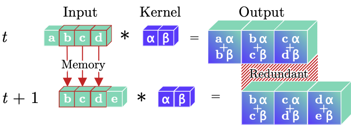
(1)
Regular Convolution. A regular temporal convolutional layer leads to redundant computations during online processing of video clips, as illustrated by the repeated convolution of inputs (green b,c,d) with a kernel (blue α,β) in the temporal dimension. Moreover, prior inputs (b,c,d) must be stored between time-steps for online processing tasks.
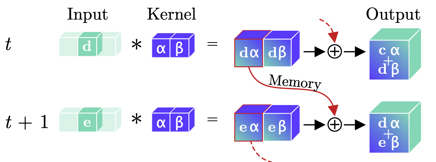
(2)
Continual Convolution. An input (green d or e) is convolved with a kernel (blue α, β). The intermediary feature-maps corresponding to all but the last temporal position are stored, while the last feature map and prior memory are summed to produce the resulting output. For a continual stream of inputs, Continual Convolutions produce identical outputs to regular convolutions.
Comparing Figures (1) and (2), we see that Continual Convolutions get rid of computational redundancies. This can speed up online inference greatly - for example, a Continual X3D model for Human Activity Recognition has 10× less Floating Point Operations per prediction than the vanilla X3D models 🚀.
💡 The longer the length of the temporal sequence, the larger the savings.
For more information, we refer to the paper on Continual Convolutions.
Forward modes
The library components feature three distinct forward modes, which are handy for different situations, namely forward, forward_step, and forward_steps:
forward
Performs a full forward computation exactly as the regular layer would. This method is handy for effient training on clip-based data.
         O            (O: output)
         ↑
         N            (N: nework module)
         ↑
 -----------------    (-: aggregation)
 P   I   I   I   P    (I: input frame, P: padding)
forward_step
Performs a forward computation for a single frame and continual states are updated accordingly. This is the mode to use for continual inference.
O+S O+S O+S O+S   (O: output, S: updated internal state)
 ↑   ↑   ↑   ↑
 N   N   N   N    (N: nework module)
 ↑   ↑   ↑   ↑
 I   I   I   I    (I: input frame)
forward_steps
Performs a layer-wise forward computation using the continual module.
The computation is performed frame-by-frame and continual states are updated accordingly.
The output-input mapping the exact same as that of a regular module.
This mode is handy for initialising the network on a whole clip (multipleframes) before the forward is usead for continual inference.
         O            (O: output)
         ↑
 -----------------    (-: aggregation)
 O  O+S O+S O+S  O    (O: output, S: updated internal state)
 ↑   ↑   ↑   ↑   ↑
 N   N   N   N   N    (N: nework module)
 ↑   ↑   ↑   ↑   ↑
 P   I   I   I   P    (I: input frame, P: padding)
Modules
Below is a list of the included modules and utilities included in the library:
-
Convolutions:
co.Conv1dco.Conv2dco.Conv3d
-
Pooling:
co.AvgPool1dco.AvgPool2dco.AvgPool3dco.MaxPool1dco.MaxPool2dco.MaxPool3dco.AdaptiveAvgPool1dco.AdaptiveAvgPool2dco.AdaptiveAvgPool3dco.AdaptiveMaxPool1dco.AdaptiveMaxPool2dco.AdaptiveMaxPool3d
-
Containers
co.Sequential- Sequential wrapper for modules. This module automatically performs conversions of torch.nn modules, which are safe during continual inference. These include all batch normalisation and activation function.co.Parallel- Parallel wrapper for modules.co.Residual- Residual wrapper for modules.co.Delay- Pure delay module (e.g. needed in residuals).
-
Converters
co.continual- conversion function fromtorch.nnmodules tocomodules.co.forward_stepping- functional wrapper, which enhances temporally localtorch.nnmodules with the forward_stepping functions.
In addition, we support interoperability with a wide range of modules from torch.nn:
-
Activation
nn.BatchNorm1dnn.Thresholdnn.ReLUnn.RReLUnn.Hardtanhnn.ReLU6nn.Sigmoidnn.Hardsigmoidnn.Tanhnn.SiLUnn.Hardswishnn.ELUnn.CELUnn.SELUnn.GLUnn.GELUnn.Hardshrinknn.LeakyReLUnn.LogSigmoidnn.Softplusnn.Softshrinknn.PReLUnn.Softsignnn.Tanhshrinknn.Softminnn.Softmaxnn.Softmax2dnn.LogSoftmax
-
Batch Normalisation
nn.BatchNorm1dnn.BatchNorm2dnn.BatchNorm3d
-
Dropout
nn.Dropoutnn.Dropout2dnn.Dropout3dnn.AlphaDropoutnn.FeatureAlphaDropout
Advanced examples
Continual 3D MBConv
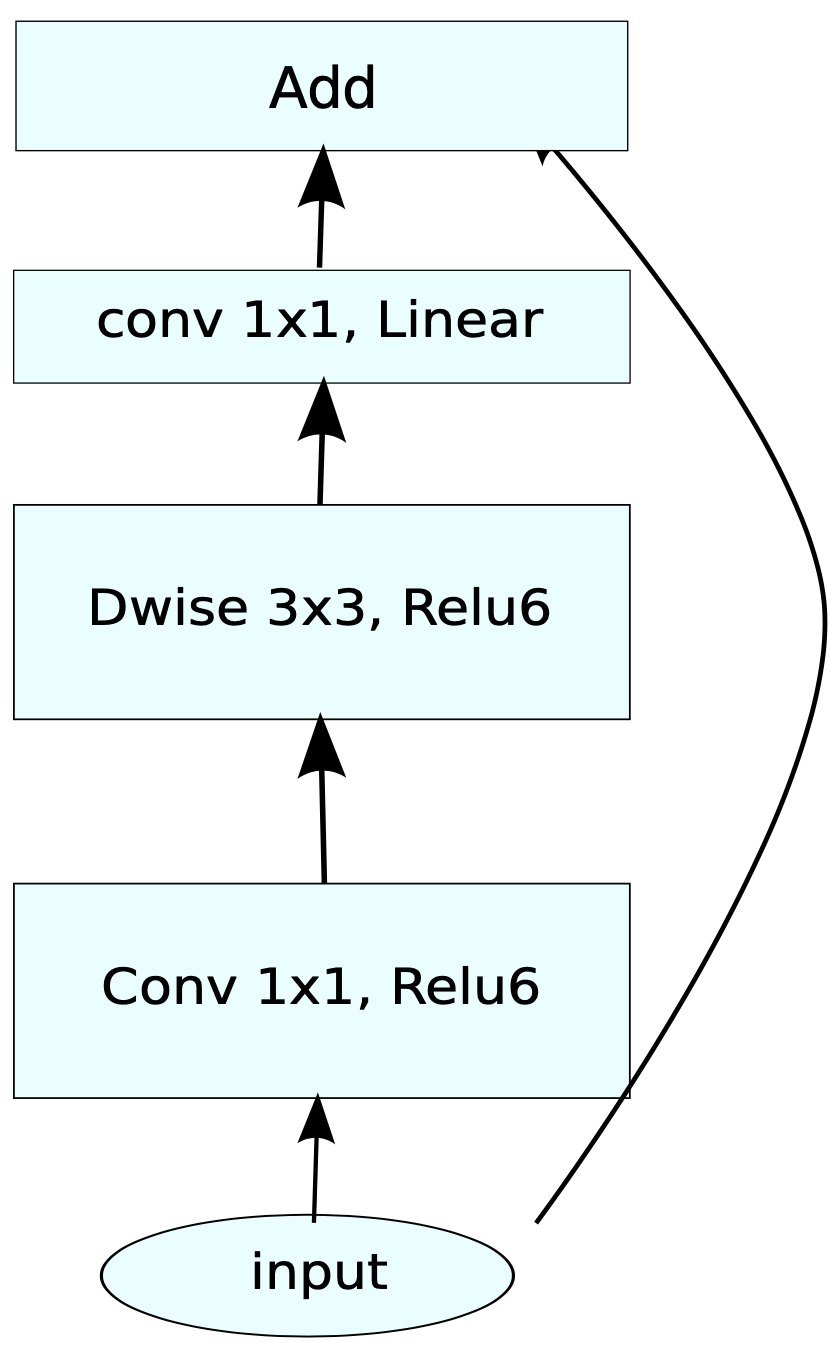
MobileNetV2 Inverted residual block. Source: https://arxiv.org/pdf/1801.04381.pdf
mb_conv = co.Residual(
    co.Sequential(
      co.Conv3d(32, 64, kernel_size=(1, 1, 1)),
      nn.BatchNorm3d(64),
      nn.ReLU6(),
      co.Conv3d(64, 64, kernel_size=(3, 3, 3), padding=(1, 1, 1), groups=64),
      nn.ReLU6(),
      co.Conv3d(64, 32, kernel_size=(1, 1, 1)),
      nn.BatchNorm3d(32),
    )
)
Continual 3D Inception module
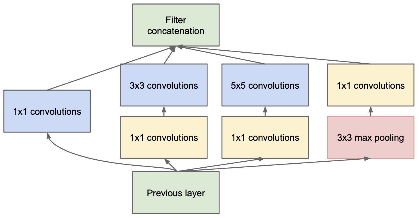
Inception module with dimension reductions. Source: https://arxiv.org/pdf/1409.4842v1.pdf
def norm_relu(module, channels):
    return co.Sequential(
        module,
        nn.BatchNorm3d(channels),
        nn.ReLU(),
    )

inception_module = co.Parallel(
    co.Conv3d(192, 64, kernel_size=1),
    co.Sequential(
        norm_relu(co.Conv3d(192, 96, kernel_size=1), 96),
        norm_relu(co.Conv3d(96, 128, kernel_size=3, padding=1), 128),
    ),
    co.Sequential(
        norm_relu(co.Conv3d(192, 16, kernel_size=1), 16),
        norm_relu(co.Conv3d(16, 32, kernel_size=3, padding=1), 32),
    ),
    co.Sequential(
        co.MaxPool3d(kernel_size=(1, 3, 3), padding=(0, 1, 1), stride=1),
        norm_relu(co.Conv3d(192, 32, kernel_size=1), 32),
    ),
    aggregation_fn="concat",
)
Continual 3D Squeeze-and-Excitation module
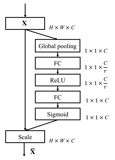
Squeeze-and-Excitation block. Scale refers to a broadcasted element-wise multiplication. Adapted from: https://arxiv.org/pdf/1709.01507.pdf
se = co.Residual(
    co.Sequential(
        OrderedDict([
            ("pool", co.AdaptiveAvgPool3d((1, 1, 1), kernel_size=7)),
            ("down", co.Conv3d(256, 16, kernel_size=1)),
            ("act1", nn.ReLU()),
            ("up", co.Conv3d(16, 256, kernel_size=1)),
            ("act2", nn.Sigmoid()),
        ])
    ),
    aggregation_fn="mul",
)
Compatibility
The library modules are built to integrate seamlessly with other PyTorch projects. Specifically, extra care was taken to ensure out-of-the-box compatibility with:
Citations
This library
@article{hedegaard2021colib,
  title={Continual Inference Library},
  author={Lukas Hedegaard},
  journal={GitHub. Note: https://github.com/LukasHedegaard/continual-inference},
  year={2021}
}

@article{hedegaard2021co3d,
  title={Continual 3D Convolutional Neural Networks for Real-time Processing of Videos},
  author={Lukas Hedegaard and Alexandros Iosifidis},
  journal={preprint, arXiv:2106.00050},
  year={2021}
}
Release history Release notifications | RSS feed


Download files
Download the file for your platform. If you're not sure which to choose, learn more about installing packages.
Source Distribution
Built Distribution
Filter files by name, interpreter, ABI, and platform.
If you're not sure about the file name format, learn more about wheel file names.
Copy a direct link to the current filters
File details
Details for the file continual-inference-0.7.0.tar.gz.
File metadata
- Download URL: continual-inference-0.7.0.tar.gz
- Upload date:
- Size: 26.2 kB
- Tags: Source
- Uploaded using Trusted Publishing? No
- Uploaded via: twine/3.4.2 importlib_metadata/4.6.4 pkginfo/1.7.1 requests/2.26.0 requests-toolbelt/0.9.1 tqdm/4.62.2 CPython/3.7.11
File hashes
| Algorithm | Hash digest | |
|---|---|---|
| SHA256 |
761bdfc46caa9d918a9905a696745fc8a9ee84f9335bb5f001b9860fe5b145c1
|
|
| MD5 |
7eceaf5e2dc1e45fb4043736b0c5bcbc
|
|
| BLAKE2b-256 |
9258606762c7347c6f5adf7039d287f2b66911c32882a4c4eb7a293d483dd5eb
|
File details
Details for the file continual_inference-0.7.0-py3-none-any.whl.
File metadata
- Download URL: continual_inference-0.7.0-py3-none-any.whl
- Upload date:
- Size: 29.3 kB
- Tags: Python 3
- Uploaded using Trusted Publishing? No
- Uploaded via: twine/3.4.2 importlib_metadata/4.6.4 pkginfo/1.7.1 requests/2.26.0 requests-toolbelt/0.9.1 tqdm/4.62.2 CPython/3.7.11
File hashes
| Algorithm | Hash digest | |
|---|---|---|
| SHA256 |
4f2902b8612f527986a8d164c3980f7394c96524612713050931b3ae952b22dd
|
|
| MD5 |
a3f4b3d59eaa92c2e33198a7b5708d01
|
|
| BLAKE2b-256 |
73807e8db23f91657125e2f6482491145e19430dc0c7507ead057cb7c43a8aa5
|


