

Numerical continuation of nonlinear equilibrium equations.






Contique is a Python 3.10+ package that provides methods for numeric continuation.
✨ Highlights
Contique's
- ✅ powerful numeric continuation method
contique.solve()
is best classified as a
- ✅ component-based continuation with an
- ✅ adaptive magnitude-based control-component switching.
📦 Installation
Install Python, open a terminal and run
pip install contique
Contique depends on
numpy(for arrays) andscipy(check if matrix is sparse and for a sparse solver).
🚀 Getting Started
A given set of equilibrium equations in terms of x and lpf (a.k.a. load-proportionality-factor) should be solved by numeric continuation of a given initial solution. Let's choose a function
import numpy as np

def fun(x, lpf, a, b):
    return np.array(
        [-a * np.sin(x[0]) + x[1] ** 2 + lpf, -b * np.cos(x[1]) * x[1] + lpf]
    )
with its initial solution and function parameters.
x0 = np.zeros(2)
lpf0 = 0.0

a = 1
b = 1
Now let's run contique.solve() and plot the states of equilibrium.
import contique

res = contique.solve(
    fun=fun,
    x0=x0,
    args=(a, b),
    lpf0=lpf0,
    dxmax=0.1,
    dlpfmax=0.1,
    maxsteps=75,
    maxcycles=4,
    maxiter=20,
    tol=1e-8,
    overshoot=1.05,
)
For each step a summary is printed out per cycle. This contains an information about the control component at the beginning and the end of a cycle as well as the norm of the residuals along with needed Newton-Rhapson iterations per cycle. As an example the ouput of some interesting steps 31-33 and 38-40 are shown below. The last column contains messages about the solution. On the one hand, in step 32, cycle 1 the control component changed from +1 to -2, but the relative overshoot on the final control component -2 was inside the tolerated range of overshoot=1.05. Therefore the solver proceeds with step 33 without re-cycling step 32. On the other hand, in step 39, cycle 1 the control component changed from -2 to -1 and this time the overshoot on the final control component -1 was outside the tolerated range. A new cycle 2 is performed for step 39 with the new control component -1.
|Step,C.| Control Comp. | Norm (Iter.#) | Message     |
|-------|---------------|---------------|-------------|

(...)

|  31,1 |   +1  =>   +1 | 7.6e-10 ( 3#) |             |
|  32,1 |   +1  =>   -2 | 1.7e-14 ( 4#) |tol.Overshoot|
|  33,1 |   -2  =>   -2 | 4.8e-12 ( 3#) |             |

 (...)

|  38,1 |   -2  =>   -2 | 9.2e-12 ( 3#) |             |
|  39,1 |   -2  =>   -1 | 1.9e-13 ( 3#) | => re-Cycle |
|     2 |   -1  =>   -1 | 2.3e-13 ( 4#) |             |
|  40,1 |   -1  =>   -1 | 7.9e-09 ( 3#) |             |

(...)
Next, we have to assemble the results
X = np.array([r.x for r in res])
and plot the solution curve.
import matplotlib.pyplot as plt

plt.plot(X[:, 0], X[:, 1], "C0.-")
plt.xlabel(r"$x_1$")
plt.ylabel(r"$x_2$")
plt.plot([0], [0], "C0o", lw=3)
plt.arrow(
    X[-2, 0],
    X[-2, 1],
    X[-1, 0] - X[-2, 0],
    X[-1, 1] - X[-2, 1],
    head_width=0.075,
    head_length=0.15,
    fc="C0",
    ec="C0",
)
plt.gca().set_aspect("equal")
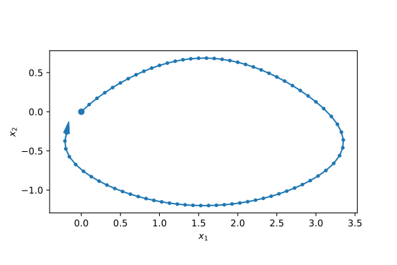
Fig. 1 Solution states of equilibrium equations solved with contique.
📝 A Brief Theory Guide - Numeric Continuation
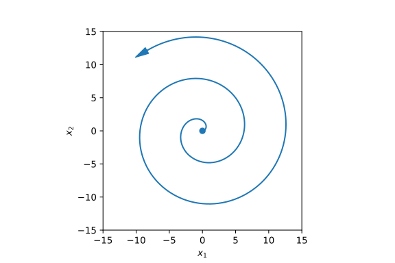
Fig. 2 Archimedean spiral equation solved with contique.
Extended Equilibrium Equations
The lpf value is appended to the unknows x which gives the so-called extended unknowns y = [x, lpf]. One additional control equation is added to the equilibrium equations to ensure (n+1) equations in terms of (n+1) extended unknowns (see next section). This reduces the solution to a point on the initial solution curve.
Control Equation
The control equation is defined as follows: First, a needle-vector with dimension (n+1) is created and filled with zeros needle = 0. For a given initial signed control component j the needle is positioned at needle[|j|] = 1. The maximum allowed values per component are calculated as ymax = y0 + np.sign(j) dymax. The control equation is finally formulated as f(y) = needle.T (y - ymax).
Solution Technique
The numeric solution process is divided into three main parts:
- Step
- Cycle
- Iteration (...of a Newton-Rhapson root method)
- Cycle
As the name implies, a Step tries to find the extended unknowns for the next step forward of the equilibrium state. For each Cycle, the initial control component has to be evaluated first (see comment below). The additional control equation is evaluated with this initial control component. The generated extended equilibrium equations in terms of the extended unknows are now solved with the help of a root method (Newton-Rhapson Iterations). The solution of the root method dy is further normalized as dy/dymax and the final control component is evaluated as j = |j| sign((dy/dymax)[|j|]) with |j| = argmax(|dy/dymax|). If the control component changed, another Cycle is performed with the initial control component being now the final control component of the last cycle. This Cycle-loop is repeated until the control component does not change anymore.
Note Pre-evaluation of the initial control component of a Step: This is performed by the linear solution of the extended equilibrium equations. It is equal to the result of the first Iteration of the Newton-Rhapson root method.
🛠️ Testing
To run the contique unit tests, check out this repository and type
tox
📄 Changelog
All notable changes to this project will be documented in this file. The format is based on Keep a Changelog, and this project adheres to Semantic Versioning.
🔓 License
Contique - Numerical continuation of nonlinear equilibrium equations (C) 2021-2025 Andreas Dutzler, Graz (Austria).
This program is free software: you can redistribute it and/or modify it under the terms of the GNU General Public License as published by the Free Software Foundation, either version 3 of the License, or (at your option) any later version.
This program is distributed in the hope that it will be useful, but WITHOUT ANY WARRANTY; without even the implied warranty of MERCHANTABILITY or FITNESS FOR A PARTICULAR PURPOSE. See the GNU General Public License for more details.
You should have received a copy of the GNU General Public License along with this program. If not, see https://www.gnu.org/licenses/.
1 maintainer

Metadata
1 maintainer
Release files for contique 1.1.1
For a detailed explanation of source distributions (sdists) and built distributions (wheels), please see the package formats documentation.
Source distribution (sdist)
| File | Size | Uploaded | |
|---|---|---|---|
| contique-1.1.1.tar.gz | 28.7 kB | Details |
Built distribution (wheel)
| File | Interpreter | ABI | Platform | Reset |
|---|---|---|---|---|
| contique-1.1.1-py3-none-any.whl | Python 3 | none | any | Details |
Total release size: 55.2 kB
Release files / contique-1.1.1.tar.gz
| Download URL | contique-1.1.1.tar.gz |
|---|---|
| Size | 28.7 kB |
| Tags | Source |
|
SHA-256 checksum How to use checksums |
68172490e9dde9f07177d8cfbb4b7439a17d2af1ce3ab7206d91baa9463d69ee
|
|
BLAKE2b-256 checksum How to use checksums |
7b895367ab1debd21c1dfacad99c68db17b59bd6a462c3bb71c30a9ef64f4cd2
|
| Upload date | |
|
Uploaded using Trusted Publishing? What is trusted publishing? |
No |
| Uploaded via |
twine/6.1.0 CPython/3.13.7
|
Release files / contique-1.1.1-py3-none-any.whl
| Download URL | contique-1.1.1-py3-none-any.whl |
|---|---|
| Size | 26.5 kB |
| Tags | Python 3 |
|
SHA-256 checksum How to use checksums |
549cd2af6565c6647f8a1812281ec7d7e1ea6902caeb50b504bf8495083e2a42
|
|
BLAKE2b-256 checksum How to use checksums |
2b39742893ed8ee1184291991b01967c7d6b0f4f01e598a9047ad17cbf4f3210
|
| Upload date | |
|
Uploaded using Trusted Publishing? What is trusted publishing? |
No |
| Uploaded via |
twine/6.1.0 CPython/3.13.7
|














