
controlchartspy
The controlchartspy package provides tools for both calculating and visualising
statistical process control (SPC), funnel, and multi-indicator sigma charts in
Python. It is based on the R
controlcharts package.
Installation
Install from PyPi with:
uv add controlchartspy
Or install the development version from GitHub with:
uv add --git https://github.com/AUS-DOH-Safety-and-Quality/controlchartspy/
Getting Started
Constructing SPC Charts
Consider a basic time series comprising two years of monthly data:
from datetime import date
from random import Random

from controlchartspy import spc, funnel

rng = Random(12324)
dat = {
    "month": [date(2024 + i // 12, i % 12 + 1, 1) for i in range(24)],
    "y": [rng.gauss(0, 1) for _ in range(24)],
}
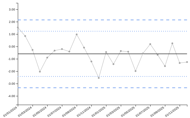
By default, the spc() function constructs an i-chart (individuals chart,
also referred to as an XmR chart):
spc_chart = spc(data=dat, keys="month", numerators="y")
The result is a ControlChart containing:
static_plot: a static SVG plot of the SPC chart.limits: a list of records containing the calculated control limits.
Display the plot in a notebook:
spc_chart.static_plot
Inspect the first three limit records:
from pprint import pprint

pprint(spc_chart.limits[:3], sort_dicts=False)
[{'date': '01/01/2024',
  'value': 1.5421097574859834,
  'target': -0.594252476265739,
  'll99': -3.336604002943138,
  'll95': -2.422486827384005,
  'll68': -1.508369651824872,
  'ul68': 0.3198646992933941,
  'ul95': 1.2339818748525273,
  'ul99': 2.1480990504116604,
  'trend_line': -0.0438723999116986},
 {'date': '01/02/2024',
  'value': 0.8450795313134178,
  'target': -0.594252476265739,
  'll99': -3.336604002943138,
  'll95': -2.422486827384005,
  'll68': -1.508369651824872,
  'ul68': 0.3198646992933941,
  'ul95': 1.2339818748525273,
  'ul99': 2.1480990504116604,
  'trend_line': -0.09173153698596298},
 {'date': '01/03/2024',
  'value': -0.27791938061152177,
  'target': -0.594252476265739,
  'll99': -3.336604002943138,
  'll95': -2.422486827384005,
  'll68': -1.508369651824872,
  'ul68': 0.3198646992933941,
  'ul95': 1.2339818748525273,
  'ul99': 2.1480990504116604,
  'trend_line': -0.13959067406022735}]
Funnel Plot
The same interface is provided for funnel charts. For this example, consider proportion data recorded by ten organisations:
funnel_data = {
    "organisation": list("abcdefghij"),
    "numerators": [27, 23, 35, 26, 38, 22, 46, 26, 27, 35],
    "denominators": [170, 122, 178, 184, 161, 105, 190, 121, 137, 197],
}
For funnel plots, the default is a proportions (PR) chart:
funnel_chart = funnel(
    data=funnel_data,
    keys="organisation",
    numerators="numerators",
    denominators="denominators",
)
funnel_chart.static_plot
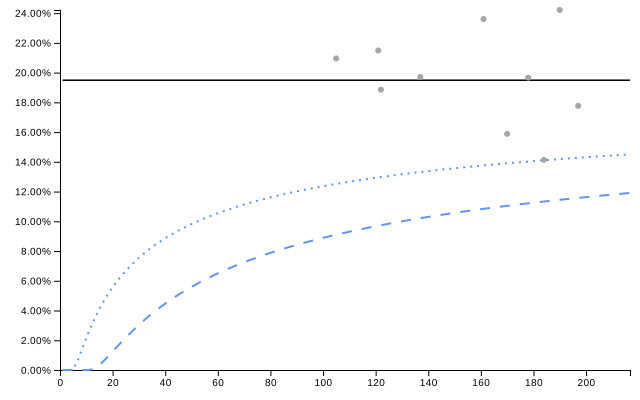
Inspect the first three limit records. Values and limits are percentages; records are ordered by denominator.
pprint(funnel_chart.limits[:3], sort_dicts=False)
[{'denominator': 105,
  'group': 'f',
  'numerator': 22,
  'value': 20.952380952380953,
  'z': 0.3734456258038048,
  'target': 19.488817891373802,
  'll99': 9.100195099772012,
  'll95': 12.51476452678048,
  'll68': 15.79416361293754,
  'ul68': 23.470617415242504,
  'ul95': 27.575733596704584,
  'ul99': 32.631402897252705},
 {'denominator': 121,
  'group': 'h',
  'numerator': 26,
  'value': 21.487603305785125,
  'z': 0.5448873656525446,
  'target': 19.488817891373802,
  'll99': 9.70266069838873,
  'll95': 12.951239970877559,
  'll68': 16.03721031743157,
  'ul68': 23.189626957479458,
  'ul95': 26.992492421239433,
  'ul99': 31.66717662194669},
 {'denominator': 122,
  'group': 'b',
  'numerator': 23,
  'value': 18.852459016393443,
  'z': -0.17856345913252486,
  'target': 19.488817891373802,
  'll99': 9.736836999381445,
  'll95': 12.97581932678086,
  'll68': 16.050836651226742,
  'ul68': 23.173959368513962,
  'ul95': 26.96001503043085,
  'ul99': 31.613520185472975}]
Chart Types
The package supports fourteen SPC chart types and three funnel plot types.
Select a chart type with spc_settings={"chart_type": ...} or
funnel_settings={"chart_type": ...}:
| Function | Chart types | Additional required inputs |
|---|---|---|
spc |
run, i (default), i_m, i_mm, mr, c, g, t |
None |
spc |
p, pp (proportions), u, up (rates) |
denominators |
spc |
xbar (sample means) |
denominators, xbar_sds |
spc |
s (sample standard deviations) |
denominators; supply standard deviations as numerators |
funnel |
PR (proportions, default), SR (indirectly standardised ratios), RC (rates) |
denominators |
The individuals chart uses moving ranges to calculate control limits. i_m
uses a median centreline; i_mm also uses median moving-range limits. pp and
up are proportion and rate charts with large-sample correction.
Data and Arguments
data accepts a mapping of columns or a sequence of records. Column arguments
accept a column name or a sequence in the original row order:
keys: the categories of the chart; for SPC charts, these form the x-axis.numerators: the numeric observations for each category.denominators: the denominators for each category, where required.labels: optional labels for each category.
SPC keys accept Python date objects and ISO date strings (YYYY-MM-DD),
including mixtures in one column. Rows are sorted by key, within indicator
groups when supplied. Funnel keys identify organisations or other groups.
Numeric None and NaN values are treated as missing. Infinite values are
rejected. Repeated keys are aggregated: numerators and denominators
default to sum, while other input fields default to first. Override these
with aggregations, using first, last, sum, mean, min, max, median,
or count.
Numeric aggregations follow Power BI column aggregation: missing values are
ignored, zeros are included, and an entirely missing group stays missing.
count counts non-missing values. Numerators and denominators are aggregated
independently. first and last select by input row order, including missing values.
Aesthetic Options
Visual adjustments are handled through dedicated settings arguments. Each group
of settings has its own argument, such as canvas_settings, line_settings,
scatter_settings, x_axis_settings, or y_axis_settings. SPC charts also accept
date_settings, while label_settings controls observation labels.
To see the full list of available options, retrieve the complete defaults or one group:
from controlchartspy import spc_default_settings, funnel_default_settings

spc_defaults = spc_default_settings()
x_axis_defaults = spc_default_settings("x_axis")
funnel_defaults = funnel_default_settings("funnel")
Each settings argument is a mapping. Values can be scalars, one-element sequences, or sequences aligned with the original input rows.
For example, add a title and customise the x-axis:
styled_chart = spc(
    data=dat,
    keys="month",
    numerators="y",
    title={"text": "Monthly Performance", "font_size": "20px"},
    x_axis_settings={
        "xlimit_tick_rotation": -45,
        "xlimit_label": "Month of Observation",
    },
)
styled_chart.static_plot
Outlier Detection
Configure outlier detection through outlier_settings. SPC charts support
astronomical points, shifts, trends, and two-in-three patterns. Use
spc_default_settings("outliers") to see the available detection parameters.
NHS variation and assurance icons are configured through nhs_icon_settings.
Detection switches apply to the whole chart, separately for each SPC indicator. With row-aligned settings, the engine uses the first row with valid outlier settings after sorting and aggregating keys. Returned flag columns use those same settings.
spc_data = {
    "date": [date(2023, month, 1) for month in range(1, 13)],
    "value": [10, 12, 11, 15, 12, 11, 25, 12, 11, 10, 11, 12],
}
outlier_chart = spc(
    data=spc_data,
    keys="date",
    numerators="value",
    outlier_settings={
        "astronomical": True,
        "shift": True,
        "trend": True,
        "two_in_three": True,
    },
)
outlier_chart.static_plot
outlier_chart.limits
Phases and Grouped Limits
Use groupings to calculate separate limits for phases of one time series:
grouped_data = {
    **dat,
    "phase": ["Before"] * 12 + ["After"] * 12,
    "site": ["A"] * 12 + ["B"] * 12,
}
phased_chart = spc(
    data=grouped_data,
    keys="month",
    numerators="y",
    groupings="phase",
)
grouped_chart = spc(
    data=grouped_data,
    keys="month",
    numerators="y",
    indicators="site",
    return_objs="limits",
)
site_a_limits = grouped_chart.limits["A"]
indicators create separate series and nested limits. A mapping such as
indicators={"Region": "region", "Site": "site"} creates a nested mapping in
that order, with names available through chart.indicator_names. A single
indicator group can render a plot; multiple groups require return_objs="limits".
Multi-indicator Sigma Charts
Use misc() to compare one organisation across several indicators. Each indicator
uses an independent funnel calculation over its comparison population. The chart
shows the selected organisation's z-scores, with positive scores indicating
favourable performance.
from controlchartspy import misc

comparison = {
    "organisation": list("ABCDABCD"),
    "indicator": ["Measure A"] * 4 + ["Measure B"] * 4,
    "numerator": [8, 5, 4, 6, 2, 4, 5, 3],
    "denominator": [10] * 8,
}
sigma_chart = misc(
    comparison,
    keys="organisation",
    numerators="numerator",
    denominators="denominator",
    indicators="indicator",
    target="A",
    outlier_settings={"improvement_direction": ["increase"] * 4 + ["decrease"] * 4},
)
sigma_chart.static_plot
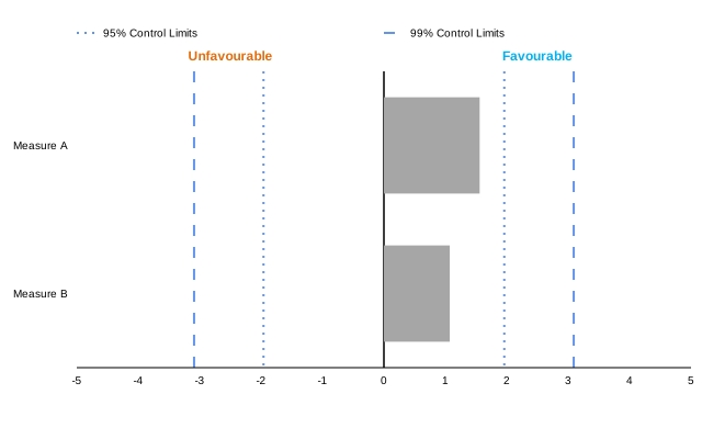
Inspect the returned records for the selected organisation:
pprint(sigma_chart.limits, sort_dicts=False)
[{'indicator': 'Measure A',
  'group': 'A',
  'z': 1.558790495298732,
  'score': 1.558790495298732,
  'three_sigma': 'none',
  'numerator': 8,
  'denominator': 10,
  'value': 80,
  'target': 57.49999999999999,
  'alt_target': None,
  'll99': 13.216714304122751,
  'll95': 27.39016233134321,
  'll68': 41.84129995477897,
  'ul68': 72.42308266420663,
  'ul95': 84.81980066370618,
  'ul99': 95.17325739282423},
 {'indicator': 'Measure B',
  'group': 'A',
  'z': -1.07140640762028,
  'score': 1.07140640762028,
  'three_sigma': 'none',
  'numerator': 2,
  'denominator': 10,
  'value': 20,
  'target': 35,
  'alt_target': None,
  'll99': 2.071914317061943,
  'll95': 10.084383484380846,
  'll68': 20.982115523920374,
  'ul68': 50.48911923810838,
  'ul95': 65.49569052552037,
  'ul99': 81.1481422890441}]
Measure B's score reverses its z-score because decreases indicate improvement.
misc() delegates to funnel() with indicators and
misc_settings={"group": target}. You can call funnel() directly with those
arguments; omitting group selects the first group. indicators accepts one
column or a mapping such as {"Domain": "domain", "Measure": "indicator"}.
Rows are sorted by indicator columns and key; indicators without the selected
target are omitted. Three-sigma outlier detection is always enabled.
All settings use the native Funnel options and align with the input rows. Each
indicator must have one improvement_direction. Use misc_settings for sigma
bounds and bar height, and outlier_settings for bar colours, such as
three_sigma_colour_improvement. misc_default_settings() returns the same
defaults as funnel_default_settings().
Results and Saving Plots
All constructors return a ControlChart. return_objs accepts one output name
or an iterable; its default is ("static_plot", "limits").
| Attribute | Contents |
|---|---|
static_plot |
StaticPlot with to_svg() and notebook SVG display |
limits |
A list of records, or nested mappings for grouped SPC series |
limit_lines |
Funnel control limits across the full range of denominators; available without indicators, by requesting "limit_lines" |
indicator_names |
SPC indicator names in nesting order |
Unrequested outputs are None. SPC records include the formatted date,
value, target, and applicable lower/upper limits (ll68, ll95, ll99,
ul68, ul95, ul99). Columns depend on chart type and requested signal flags.
Funnel records include group, numerator, denominator, value, z, target,
and limits. Proportion charts use percentage values under the default settings.
Sigma records include indicator, group, the original z, the
direction-adjusted score, three_sigma, and the corresponding funnel values
and limits. The selected organisation is recorded in group.
Save a plot as SVG with save_plot():
spc_chart.save_plot("spc_chart.svg")
funnel_chart.save_plot("funnel_chart.svg", width=960, height=600)
Specify width and height to render at a different size, or use
spc_chart.static_plot.to_svg() to get the SVG as a string. The default size is
640 × 400 pixels. Static plots display as SVGs in notebooks.
The R package documentation provides further information about the shared calculation and display settings.
1 maintainer

Metadata
1 maintainer
Release files for controlchartspy 0.1.1
For a detailed explanation of source distributions (sdists) and built distributions (wheels), please see the package formats documentation.
Source distribution (sdist)
| File | Size | Uploaded | |
|---|---|---|---|
| controlchartspy-0.1.1.tar.gz | 235.8 kB | Details |
Built distribution (wheel)
| File | Interpreter | ABI | Platform | Reset |
|---|---|---|---|---|
| controlchartspy-0.1.1-py3-none-any.whl | Python 3 | none | any | Details |
Total release size: 369.8 kB
Release files / controlchartspy-0.1.1.tar.gz
| Download URL | controlchartspy-0.1.1.tar.gz |
|---|---|
| Size | 235.8 kB |
| Tags | Source |
|
SHA-256 checksum How to use checksums |
55be5c54fb7dc6c76692ea56e443670ea558a41ff174daefa9b55272083dd05b
|
|
BLAKE2b-256 checksum How to use checksums |
0499524f989f9b188d0e506d3d53185f40abcf79ddaa221cb888e829f2ff3132
|
| Upload date | |
|
Uploaded using Trusted Publishing? What is trusted publishing? |
Yes |
| Uploaded via |
uv/0.13.0 {"installer":{"name":"uv","version":"0.13.0","subcommand":["publish"]},"python":null,"implementation":{"name":null,"version":null},"distro":{"name":"Ubuntu","version":"24.04","id":"noble","libc":null},"system":{"name":null,"release":null},"cpu":null,"openssl_version":null,"setuptools_version":null,"rustc_version":null,"ci":true}
|
Release files / controlchartspy-0.1.1-py3-none-any.whl
| Download URL | controlchartspy-0.1.1-py3-none-any.whl |
|---|---|
| Size | 134.0 kB |
| Tags | Python 3 |
|
SHA-256 checksum How to use checksums |
ac7d84acf2ec13d934d97f7d71fedf5351e2346be3d95bed5aadf6d0dc6511c2
|
|
BLAKE2b-256 checksum How to use checksums |
6d57f4a7d97b2d9759129434639cb29004f197fc068dcd2be85c43d16ce0ce0a
|
| Upload date | |
|
Uploaded using Trusted Publishing? What is trusted publishing? |
Yes |
| Uploaded via |
uv/0.13.0 {"installer":{"name":"uv","version":"0.13.0","subcommand":["publish"]},"python":null,"implementation":{"name":null,"version":null},"distro":{"name":"Ubuntu","version":"24.04","id":"noble","libc":null},"system":{"name":null,"release":null},"cpu":null,"openssl_version":null,"setuptools_version":null,"rustc_version":null,"ci":true}
|














