
coxmunk
Simple sunglint computation based on Cox & Munk model. The sunglint, sunlight reflected by the waves, induces different patterns at different spatial (or temporal) scales, as in these examples:
- (a) sea surface under gust wind conditions (reflex digital camera);
- (b) aerial photograph of the sea surface with visible surfactant filaments;
- (c) Sentinel-2A image (4 July 2015) in the 2190-nm channel, where sunglint is the most intense signal over water; the glint highlights eddies, ship wakes and wave packets;
- (d) Sentinel-3 RGB image (10 May 2016) over the eastern Mediterranean Sea, with high sunglint on the right side.
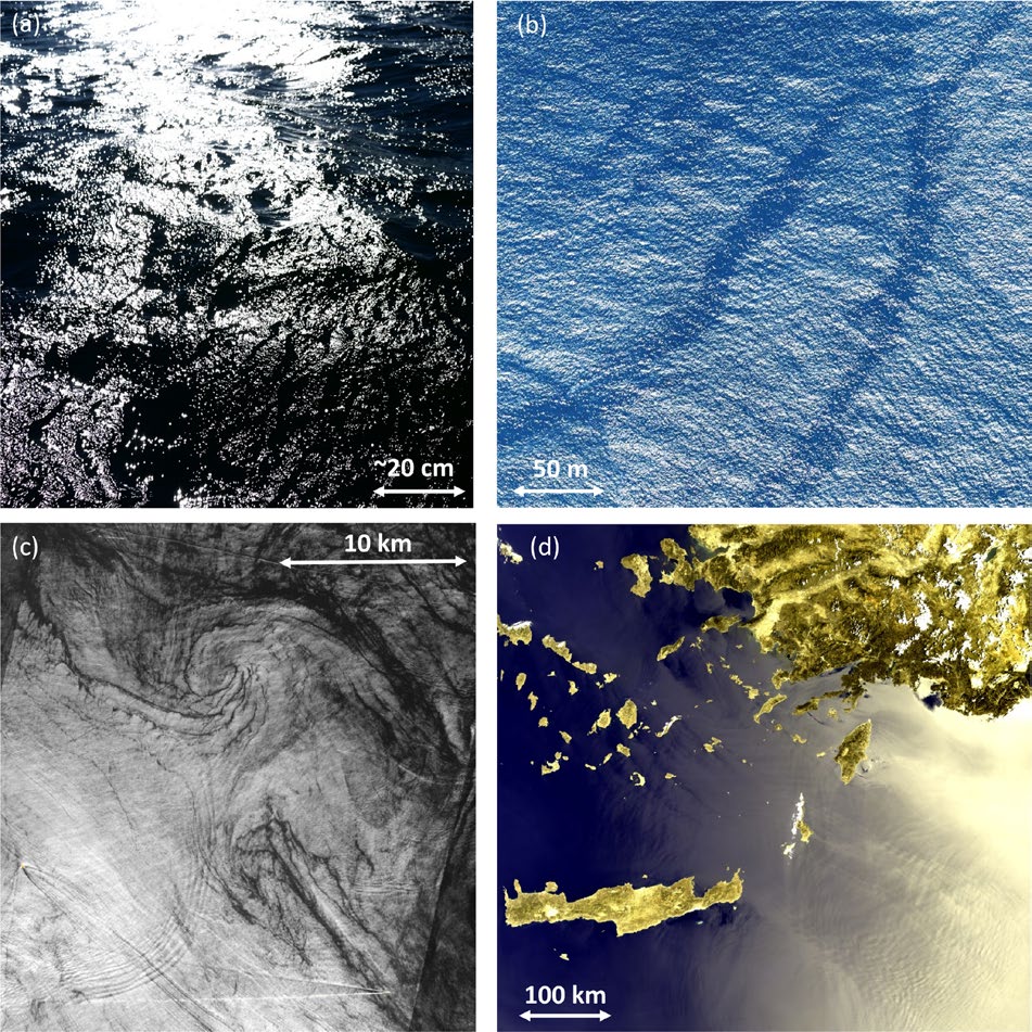
Credits: Neukermans, Harmel, Galí et al. (2018). Harnessing remote sensing to address critical science questions on ocean-atmosphere interactions. Elementa, 6, 71, doi:10.1525/elementa.331 (Fig. 11, CC BY 4.0).
For more details on the statistics of the wave slopes (i.e., Probability Distribution Function), please refer to Munk 2009.
Installation
coxmunk requires Python >= 3.9. Its dependencies (numpy, scipy, pandas, xarray, netCDF4,
matplotlib, cmocean, docopt) are installed automatically by pip.
It is best installed in a virtual environment:
python3 -m venv .venv
source .venv/bin/activate          # Windows: .venv\Scripts\activate
python -m pip install --upgrade pip
or in a conda environment:
conda create -n coxmunk python=3.12
conda activate coxmunk
From PyPI
python -m pip install coxmunk
Development version from GitHub
The develop branch contains the latest changes not yet released:
python -m pip install "git+https://github.com/Tristanovsk/coxmunk.git@develop"
From source, for development
Clone the repository and install it in editable mode (code changes are picked up without reinstalling):
git clone https://github.com/Tristanovsk/coxmunk.git
cd coxmunk
python -m pip install -e .
Run the tests with:
python -m pip install pytest
python -m pytest tests
and build the documentation with:
python -m pip install -r docs/requirements.txt
make -C docs html                  # output in docs/build/html
Check the installation
The installation provides the coxmunk command:
$ coxmunk --version
coxmunk 1.2.1
$ coxmunk
Usage:
  coxmunk <sza> <wind_speed> [--stats <stats>] [--wind_azi <wind_azi>] [--shadow] [--slope] [--figname <figname>]
  coxmunk -h | --help
  coxmunk -v | --version
The model can also be used from Python:
from coxmunk import sunglint

# geometry in degrees: solar zenith, viewing zenith, relative azimuth (180° = Sun and sensor in opposition)
I, Q, U, V = sunglint(sza=30, vza=30, azi=180).sunglint(ws=5, wazi=0, stats='bh2006', shadow=True)
The full documentation, with the API reference and tutorials, is on Read the Docs.
Model description
The sea surface is described as a collection of plane facets whose slopes follow the statistics of Cox & Munk (1954). The glint observed in a given direction comes from the facets tilted so that the Sun is specularly reflected toward the sensor.
Reflecting facet
With the solar and viewing zenith angles $\theta_s$, $\theta_v$ ($\mu = \cos\theta$) and the relative azimuth $\phi$ (180° when Sun and sensor are in opposition), the scattering angle $\Theta$, the angle of incidence on the facet $\omega$ and the facet tilt $\theta_n$ are
\cos\Theta = -\mu_s\mu_v - \sin\theta_s\sin\theta_v\cos\phi, \qquad
\omega = \frac{\pi - \Theta}{2}, \qquad
\cos\theta_n = \frac{\mu_s + \mu_v}{2\cos\omega}
The facet slopes are computed in the Sun frame and rotated into the wind frame, with $\phi_w$ the downwind direction counted counterclockwise from the Sun:
z_x = -\frac{\sin\theta_v \cos\phi + \sin\theta_s}{\mu_s + \mu_v}, \quad
z_y = -\frac{\sin\theta_v \sin\phi}{\mu_s + \mu_v}, \quad
z_{up} = \cos\phi_w \, z_x + \sin\phi_w \, z_y, \quad
z_{cr} = -\sin\phi_w \, z_x + \cos\phi_w \, z_y
Wave slope statistics
For the isotropic statistics (cm_iso), with the wind speed $U$ in m/s:
\sigma^2 = 0.003 + 5.12\times10^{-3}\,U, \qquad
P = \frac{1}{\pi\sigma^2} \exp\left(-\frac{\tan^2\theta_n}{\sigma^2}\right)
For the anisotropic statistics (cm_dir, bh2006), the Gram-Charlier expansion is written
with the convention of Munk (2009), with $\xi = z_{up}/\sigma_{up}$ and $\eta = z_{cr}/\sigma_{cr}$:
P(\xi, \eta) = \frac{e^{-(\xi^2 + \eta^2)/2}}{2\pi\,\sigma_{up}\,\sigma_{cr}}
\Big[ 1
+ \tfrac{c_{12}}{2}\,\xi\,(1 - \eta^2)
- \tfrac{c_{30}}{6}\,\xi\,(3 - \xi^2)
+ \tfrac{c_{40}}{24}\,(3 - 6\xi^2 + \xi^4)
+ \tfrac{c_{22}}{4}\,(1 - \xi^2)(1 - \eta^2)
+ \tfrac{c_{04}}{24}\,(3 - 6\eta^2 + \eta^4)
\Big]
where $c_{12} = -c_{21}$ and $c_{30} = -c_{03}$, with the coefficients:
| Parameter | cm_dir (Cox & Munk, 1954) |
bh2006 (Bréon & Henriot, 2006) |
|---|---|---|
| $\sigma_{cr}^2$ | $0.003 + 1.92\times10^{-3},U$ | $0.003 + 1.85\times10^{-3},U$ |
| $\sigma_{up}^2$ | $3.16\times10^{-3},U$ | $0.001 + 3.16\times10^{-3},U$ |
| $c_{21}$ | $0.01 - 8.6\times10^{-3},U$ | $-9\times10^{-4},U^2$ |
| $c_{03}$ | $0.04 - 0.033,U$ | $-0.45 / (1 + e^{7 - U})$ |
| $c_{40}$ | 0.40 | 0.30 |
| $c_{22}$ | 0.12 | 0.12 |
| $c_{04}$ | 0.23 | 0.40 |
Fresnel reflection
With the refractive index of water $m$ (default 1.334), the reflection coefficients parallel and perpendicular to the plane of incidence are
r_l = \frac{\sqrt{m^2 - \sin^2\omega} - m^2\cos\omega}{\sqrt{m^2 - \sin^2\omega} + m^2\cos\omega},
\qquad
r_r = \frac{\cos\omega - \sqrt{m^2 - \sin^2\omega}}{\cos\omega + \sqrt{m^2 - \sin^2\omega}}
giving the Mueller reflection matrix
\mathbf{R}_F(\omega) = \frac{1}{2}
\begin{pmatrix}
r_l^2 + r_r^2 & r_l^2 - r_r^2 & 0 & 0 \\
r_l^2 - r_r^2 & r_l^2 + r_r^2 & 0 & 0 \\
0 & 0 & 2 r_l r_r & 0 \\
0 & 0 & 0 & 2 r_l r_r
\end{pmatrix}
which is rotated from the meridian planes into the scattering plane, $\mathbf{R} = \mathbf{L}(\pi - \sigma_2),\mathbf{R}_F,\mathbf{L}(-\sigma_1)$.
Shadowing and hiding
With --shadow (shadow=True in Python), the facets hidden by the waves are removed
with the Smith function (Ross & Dion, 2005, 2007):
\Lambda(\theta, \varphi) = \frac{e^{-\nu^2} - \nu\sqrt{\pi}\,\mathrm{erfc}(\nu)}{2\,\nu\sqrt{\pi}},
\qquad
\nu = \frac{1}{\sqrt{2}\,\sigma(\varphi)\tan\theta},
\qquad
\sigma^2(\varphi) = \sigma_{up}^2\cos^2\varphi + \sigma_{cr}^2\sin^2\varphi
SH = \frac{1}{1 + \Lambda(\theta_s, -\phi_w) + \Lambda(\theta_v, \phi - \phi_w)}
where $\varphi$ is the azimuth of the direction relative to the upwind axis.
Sunglint Stokes vector
The sunglint, in reflectance units, is finally
\begin{pmatrix} I \\ Q \\ U \\ V \end{pmatrix}
= \frac{\pi \, P \, SH}{4 \, \mu_s \, \mu_v \cos^4\theta_n}
\begin{pmatrix} R_{11} \\ R_{21} \\ R_{31} \\ R_{41} \end{pmatrix}
References
- Cox, C. and Munk, W. (1954). Measurement of the roughness of the sea surface from photographs of the Sun's glitter. J. Opt. Soc. Am., 44(11), 838-850.
- Bréon, F.-M. and Henriot, N. (2006). Spaceborne observations of ocean glint reflectance and modeling of wave slope distributions. J. Geophys. Res., 111, C06005.
- Munk, W. (2009). An inconvenient sea truth: spread, steepness, and skewness of surface slopes. Annu. Rev. Mar. Sci., 1, 377-415.
- Ross, V., Dion, D. and Potvin, G. (2005). Detailed analytical approach to the Gaussian surface bidirectional reflectance distribution function specular component applied to the sea surface. J. Opt. Soc. Am. A, 22(11), 2442-2453.
- Harmel, T. and Chami, M. (2012). Determination of sea surface wind speed using the polarimetric and multidirectional properties of satellite measurements in visible bands. Geophys. Res. Lett., 39, L19611, doi:10.1029/2012GL053508.
- Harmel, T. and Chami, M. (2013). Estimation of the sunglint radiance field from optical satellite imagery over open ocean: multidirectional approach and polarization aspects. J. Geophys. Res. Oceans, 118, doi:10.1029/2012JC008221.
- Ross, V. and Dion, D. (2007). Sea surface slope statistics derived from Sun glint radiance measurements and their apparent dependence on sensor elevation. J. Geophys. Res., 112, C09015.
Polarization and wind speed retrieval
Since the polarization of the glint only depends on the geometry while its amount depends on the
sea state, multidirectional and polarized measurements (e.g., POLDER/PARASOL) can be used to
retrieve the sunglint Stokes vector (Harmel & Chami, 2013) and the sea surface wind speed
(Harmel & Chami, 2012). The coxmunk.wind module implements the forward model (sunglint plus
whitecaps) and the Levenberg-Marquardt inversion of Harmel & Chami (2012):
import numpy as np
from coxmunk.wind import glint_whitecap, retrieve_wind_speed

# 14 viewing directions along a satellite track: (sza, vza, azi) in degrees
geometries = np.array([(30, abs(v), 150 if v >= 0 else 330) for v in np.linspace(-55, 55, 14)])
observed = glint_whitecap(geometries, ws=8)          # synthetic I, Q, U measurements
res = retrieve_wind_speed(observed, geometries)       # -> res.ws, res.sigma, res.flag
See the polarization and wind speed chapters of the documentation.
Kumatage: from noise to signal
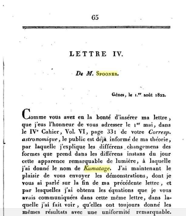
In 1822, Spooner named Kumatage (from the Greek κυμάτων, of the waves, and αὐγή, splendour) "this remarkable appearance of light" of the Sun reflected by the waves, and established its first equations. Navigators filtered it out as a glare, painters made it a subject, Cox & Munk turned it into a measurement of the sea surface slopes, ocean color remote sensing removed it as a noise, and it is now exploited as a signal on winds, waves, currents and slicks. The History section of the documentation retraces this history (adapted from Harmel, Bary, Gernez & Morin, OCEANEXT 2019), with paintings, Cox & Munk and Sentinel-2 images.
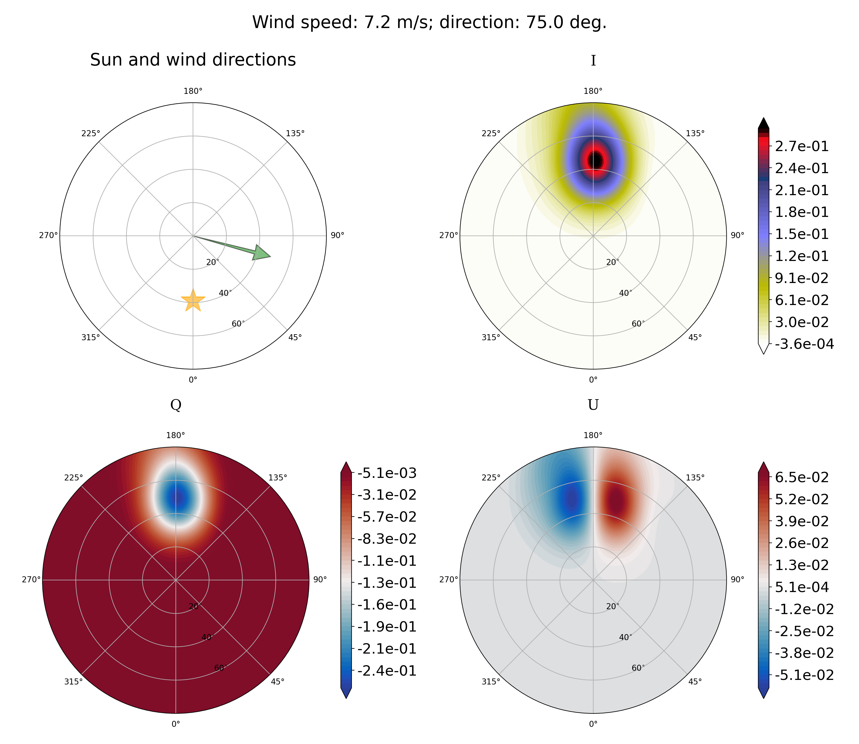
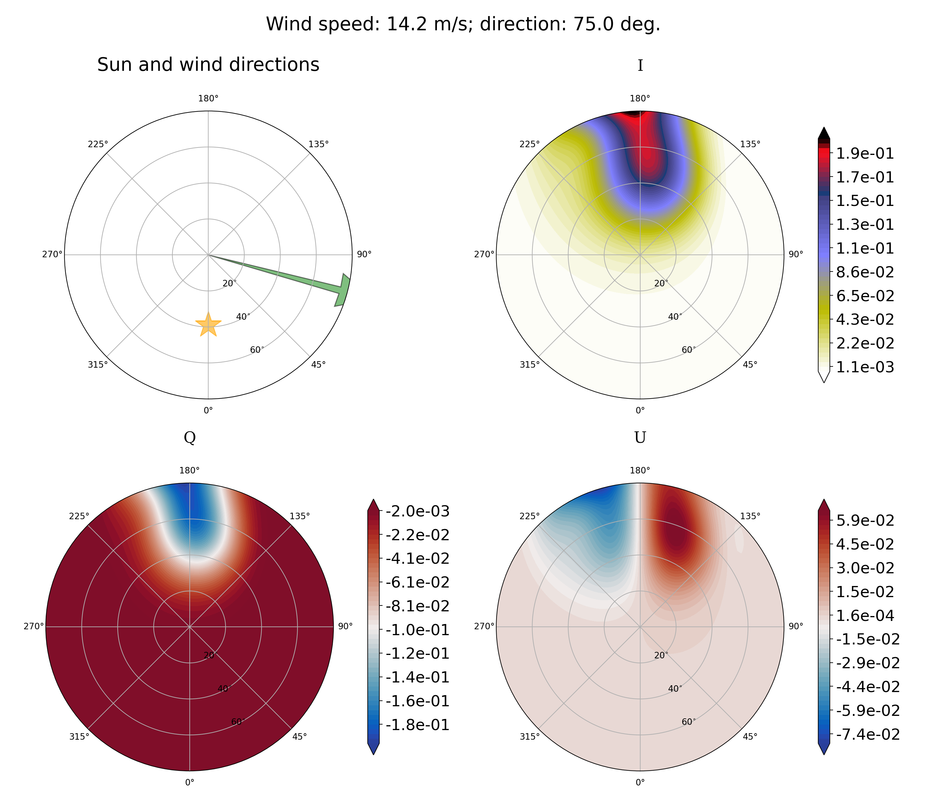
Examples
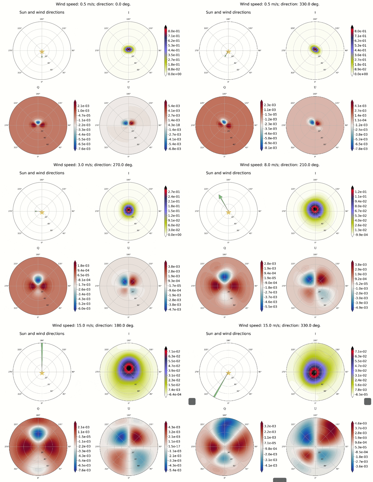
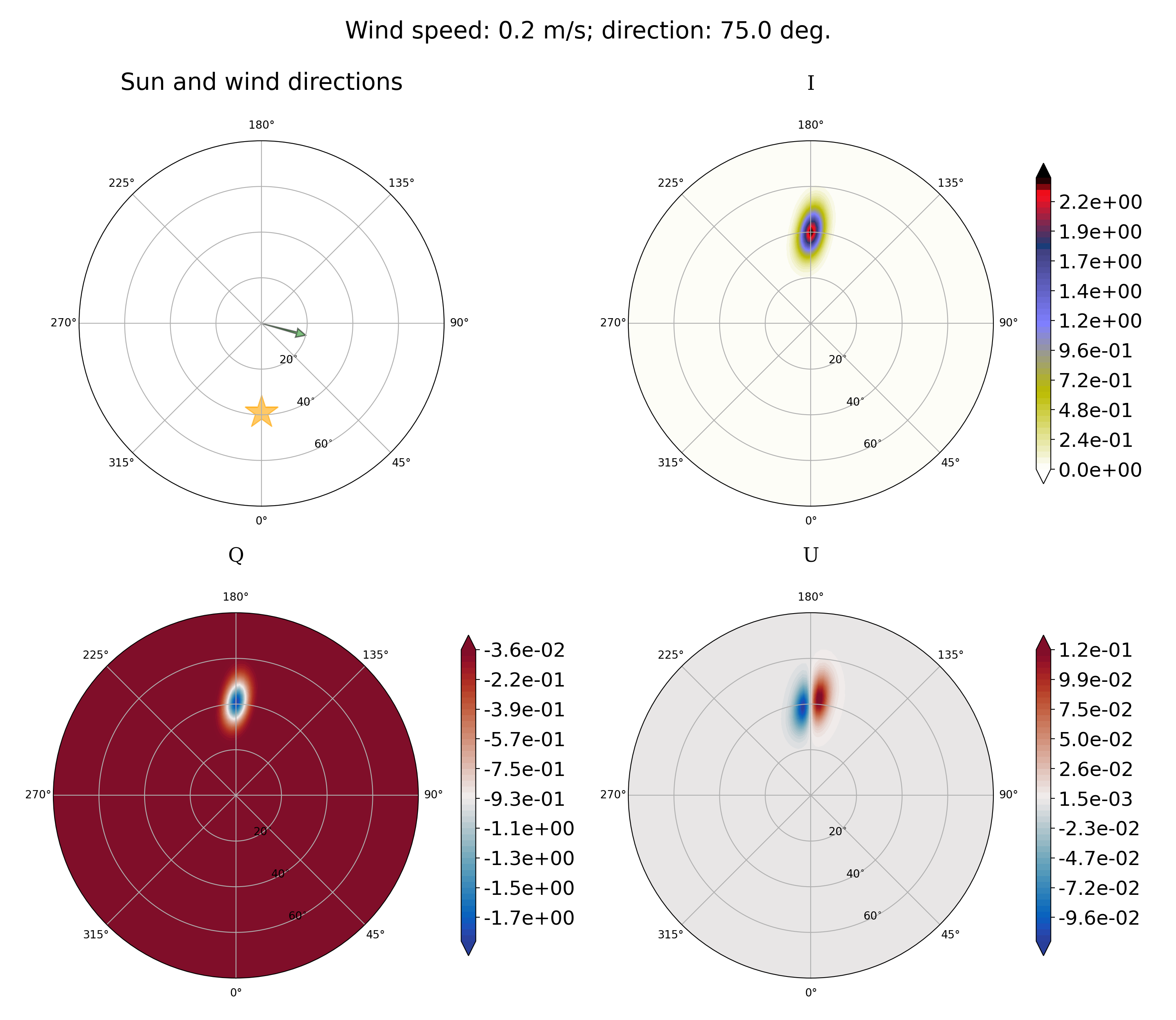
Examples for Cox & Munk model with Bréon & Henriot statistics for:
- solar zenith angle = 39°
- wind azimuth from Sun = 75°
- wind speed = 0.2, 7.2, 14.2 m.s-1
$ coxmunk 39 0.2 --stats bh2006 --wind_azi 75 --figname illustration/coxmunk_fig_39_0.2_bh2006_75.png
$ coxmunk 39 7.2 --stats bh2006 --wind_azi 75
$ coxmunk 39 14.2 --stats bh2006 --wind_azi 75
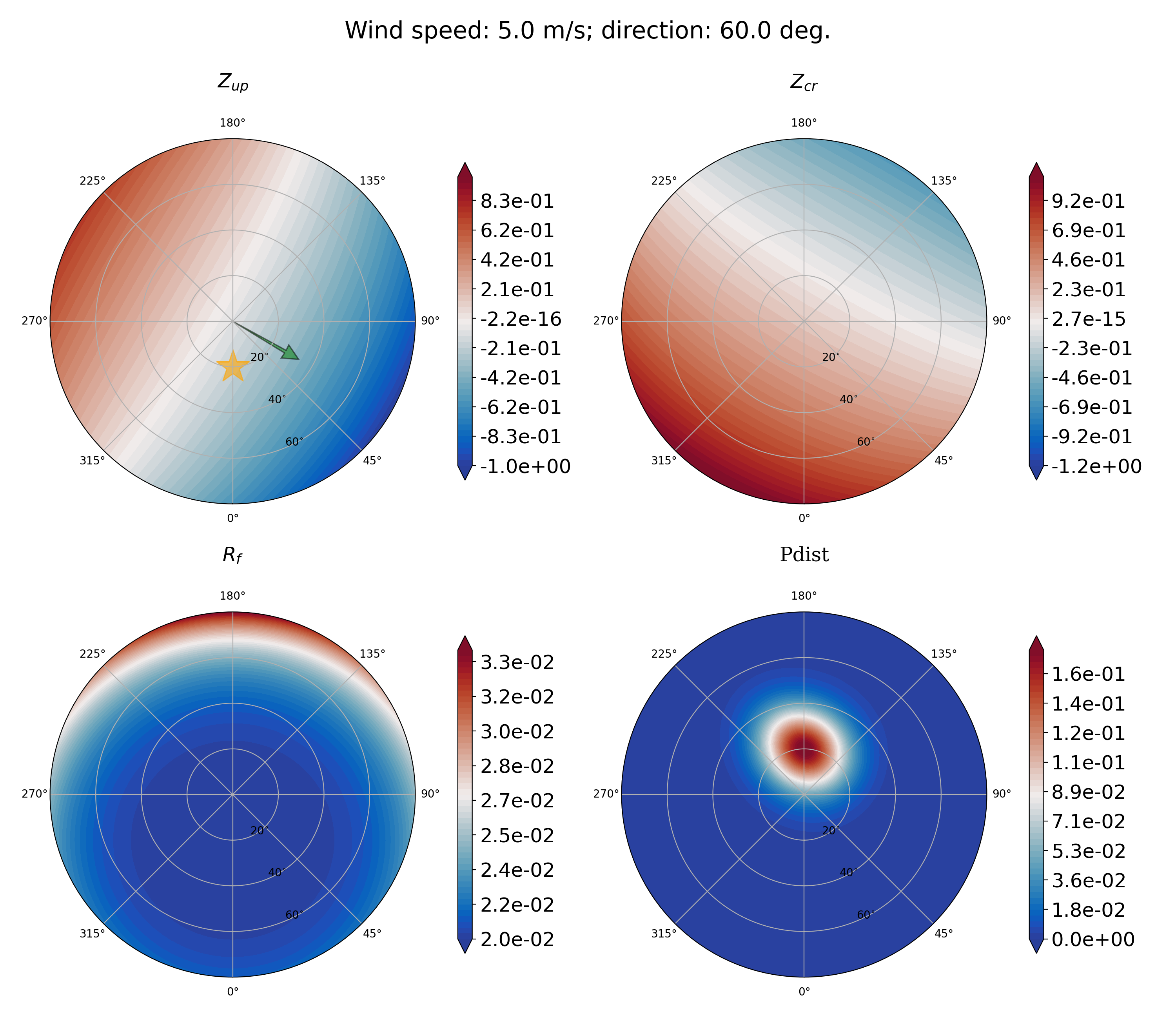
With the option --slope you can also check
the values of wave slopes upwind and crosswind,
the first term of the Fresnel matrix and the probability distribution function:
$ coxmunk 20 5 --stats bh2006 --wind_azi 60 --slope
1 maintainer

Metadata
1 maintainer
Release files for coxmunk 1.2.1
For a detailed explanation of source distributions (sdists) and built distributions (wheels), please see the package formats documentation.
Source distribution (sdist)
| File | Size | Uploaded | Provenance | |
|---|---|---|---|---|
| coxmunk-1.2.1.tar.gz | 28.3 kB | With provenance | Details |
Built distribution (wheel)
| File | Interpreter | ABI | Platform | Reset |
|---|---|---|---|---|
| coxmunk-1.2.1-py3-none-any.whl | Python 3 | none | any | Details |
Total release size: 53.6 kB
Release files / coxmunk-1.2.1.tar.gz
| Download URL | coxmunk-1.2.1.tar.gz |
|---|---|
| Size | 28.3 kB |
| Tags | Source |
|
SHA-256 checksum How to use checksums |
1b45538c8e6ab376be6aa70c8bd4a26a4bbda1d0b2426d0426a9741df74c0e9c
|
|
BLAKE2b-256 checksum How to use checksums |
f1759ca9061c9efa532fae592b83c6b4cc1ff21f2b7ade6431272427de6e0368
|
| Upload date | |
|
Uploaded using Trusted Publishing? What is trusted publishing? |
Yes |
| Uploaded via |
twine/7.0.0 CPython/3.13.16
|
Provenance
Provenance describes where a file came from. On PyPI, provenance is shared via attestations, which provide a verifiable record of the build or publishing details. View details, limitations and caveats.


PyPI Publish Attestation
PyPI verified that this artifact, at this checksum, originated from the publisher listed below.
Signed by GitHub Actions, verified by PyPI on Oct 24, 2026.
Transparency logRelease files / coxmunk-1.2.1-py3-none-any.whl
| Download URL | coxmunk-1.2.1-py3-none-any.whl |
|---|---|
| Size | 25.2 kB |
| Tags | Python 3 |
|
SHA-256 checksum How to use checksums |
bfd7078efb088f26d50a1d80f25a03fbdfdf3ef114b6fc4589b43f343a05437e
|
|
BLAKE2b-256 checksum How to use checksums |
6823f7546ad951358299196e5ded06a40ebe168ea9000f4498b3ffa4bdb33bef
|
| Upload date | |
|
Uploaded using Trusted Publishing? What is trusted publishing? |
Yes |
| Uploaded via |
twine/7.0.0 CPython/3.13.16
|
Provenance
Provenance describes where a file came from. On PyPI, provenance is shared via attestations, which provide a verifiable record of the build or publishing details. View details, limitations and caveats.
PyPI Publish Attestation
PyPI verified that this artifact, at this checksum, originated from the publisher listed below.
Signed by GitHub Actions, verified by PyPI on Oct 24, 2026.
Transparency logSecurity for coxmunk 1.2.1
Provenance
Provenance describes where a file came from. On PyPI, provenance is shared via attestations, which provide a verifiable record of the build or publishing details. View details, limitations and caveats.
Full provenance
All 2 files in this release have been uploaded with provenance metadata.
Attestation for coxmunk-1.2.1.tar.gz
PyPI Publish Attestation
PyPI verified that this artifact, at this checksum, originated from the publisher listed below.
Signed by GitHub Actions, verified by PyPI on Oct 24, 2026.
Transparency logA note on package security
PyPI is a repository for distributing packages, not a service for auditing them. While third-party security researchers and our staff do their best to detect and remove malicious packages, PyPI cannot guarantee the quality, security or suitability of any given package.
To learn more about protecting yourself from malicious actors, visit our package security documentation.













