crepes 0.6.2

Conformal classifiers, regressors, and predictive systems (crepes)

crepes is a Python package that implements conformal classifiers, regressors, and predictive systems on top of any standard classifier and regressor, turning the original predictions into well-calibrated p-values and cumulative distribution functions, or prediction sets and intervals with coverage guarantees.

The crepes package implements standard and Mondrian conformal classifiers as well as standard, normalized and Mondrian conformal regressors and predictive systems. While the package allows you to use your own functions to compute difficulty estimates, non-conformity scores and Mondrian categories, there is also a separate module, called crepes.extras, which provides some standard options for these.

Installation

From PyPI

pip install crepes

From conda-forge

conda install -c conda-forge crepes

Documentation

For the complete documentation, see crepes.readthedocs.io.

Quickstart

Let us illustrate how we may use crepes to generate and apply conformal classifiers with a dataset from www.openml.org, which we first split into a training and a test set using train_test_split from sklearn, and then further split the training set into a proper training set and a calibration set:

from sklearn.datasets import fetch_openml
from sklearn.model_selection import train_test_split

dataset = fetch_openml(name="qsar-biodeg", parser="auto")

X = dataset.data.values.astype(float)
y = dataset.target.values

X_train, X_test, y_train, y_test = train_test_split(X, y, test_size=0.5)

X_prop_train, X_cal, y_prop_train, y_cal = train_test_split(X_train, y_train,
                                                            test_size=0.25)

We now "wrap" a random forest classifier, fit it to the proper training set, and fit a standard conformal classifier through the calibrate method:

from crepes import WrapClassifier
from sklearn.ensemble import RandomForestClassifier

rf = WrapClassifier(RandomForestClassifier(n_jobs=-1))

rf.fit(X_prop_train, y_prop_train)

rf.calibrate(X_cal, y_cal)

We may now produce p-values for the test set (an array with as many columns as there are classes):

rf.predict_p(X_test)

array([[0.46552707, 0.04407598],
       [0.00382577, 0.85400826],
       [0.64930738, 0.00804963],
       ...,
       [0.33376105, 0.04065675],
       [0.16968437, 0.12810237],
       [0.02346899, 0.49634959]])

We can also get prediction sets, represented by binary vectors indicating presence (1) or absence (0) of the class labels that correspond to the columns, here at the 90% confidence level:

rf.predict_set(X_test, confidence=0.9)

array([[1, 0],
       [0, 1],
       [1, 0],
       ...,
       [1, 0],
       [1, 1],
       [0, 1]])

Since we have access to the true class labels, we can evaluate the conformal classifier (here using all available metrics which is the default):

rf.evaluate(X_test, y_test, confidence=0.9)

{'error': 0.11553030303030298,
 'avg_c': 1.0776515151515151,
 'one_c': 0.9223484848484849,
 'empty': 0.0,
 'time_fit': 2.7418136596679688e-05,
 'time_evaluate': 0.01745915412902832}

To control the error level across different groups of objects of interest, we may use so-called Mondrian conformal classifiers. A Mondrian conformal classifier is formed by providing the names of the categories as an additional argument, named bins, for the calibrate method.

Here we consider two categories formed by whether the third column (number of heavy atoms) equals zero or not:

bins_cal = X_cal[:,2] == 0

rf_mond = WrapClassifier(rf.learner)

rf_mond.calibrate(X_cal, y_cal, bins=bins_cal)

bins_test = X_test[:,2] == 0

rf_mond.predict_set(X_test, bins=bins_test)

array([[1, 0],
       [0, 1],
       [1, 0],
       ...,
       [1, 1],
       [1, 1],
       [0, 1]])

For conformal classifiers that employ learners that use bagging, like random forests, we may consider an alternative strategy to dividing the original training set into a proper training and calibration set; we may use the out-of-bag (OOB) predictions, which allow us to use the full training set for both model building and calibration. It should be noted that this strategy does not come with the theoretical validity guarantee of the above (inductive) conformal classifiers, due to that calibration and test instances are not handled in exactly the same way. In practice, however, conformal classifiers based on out-of-bag predictions rarely fail to meet the coverage requirements.

Below we show how to enable this in conjunction with a specific type of Mondrian conformal classifier, a so-called class-conditional conformal classifier, which uses the class labels as Mondrian categories:

rf = WrapClassifier(RandomForestClassifier(n_jobs=-1, n_estimators=500, oob_score=True))

rf.fit(X_train, y_train)

rf.calibrate(X_train, y_train, class_cond=True, oob=True)

rf.evaluate(X_test, y_test, confidence=0.99)

{'error': 0.009469696969697017,
 'avg_c': 1.696969696969697,
 'one_c': 0.30303030303030304,
 'empty': 0.0,
 'time_fit': 0.0002560615539550781,
 'time_evaluate': 0.06656742095947266}

Let us also illustrate how crepes can be used to generate conformal regressors and predictive systems. Again, we import a dataset from www.openml.org, which we split into a training and a test set and then further split the training set into a proper training set and a calibration set:

from sklearn.datasets import fetch_openml
from sklearn.model_selection import train_test_split

dataset = fetch_openml(name="house_sales", version=3, parser="auto")

X = dataset.data.values.astype(float)
y = dataset.target.values.astype(float)

X_train, X_test, y_train, y_test = train_test_split(X, y, test_size=0.5)
X_prop_train, X_cal, y_prop_train, y_cal = train_test_split(X_train, y_train,
                                                            test_size=0.25)

Let us now "wrap" a RandomForestRegressor from sklearn using the class WrapRegressor from crepes and fit it (in the usual way) to the proper training set:

from sklearn.ensemble import RandomForestRegressor
from crepes import WrapRegressor

rf = WrapRegressor(RandomForestRegressor())
rf.fit(X_prop_train, y_prop_train)

We may now fit a conformal regressor using the calibration set through the calibrate method:

rf.calibrate(X_cal, y_cal)

The conformal regressor can now produce prediction intervals for the test set, here using a confidence level of 99%:

rf.predict_int(X_test, confidence=0.99)

array([[-171902.2 ,  953866.2 ],
       [-276818.01,  848950.39],
       [  22679.37, 1148447.77],
       ...,
       [ 242954.02, 1368722.42],
       [-308093.73,  817674.67],
       [-227057.4 ,  898711.  ]])

The output is a NumPy array with a row for each test instance, and where the two columns specify the lower and upper bound of each prediction interval.

We may request that the intervals are cut to exclude impossible values, in this case below 0, and if we also rely on the default confidence level (0.95), the output intervals will be a bit tighter:

rf.predict_int(X_test, y_min=0)

array([[ 152258.55,  629705.45],
       [  47342.74,  524789.64],
       [ 346840.12,  824287.02],
       ...,
       [ 567114.77, 1044561.67],
       [  16067.02,  493513.92],
       [  97103.35,  574550.25]])

The above intervals are not normalized, i.e., they are all of the same size (at least before they are cut). We could make them more informative through normalization using difficulty estimates; objects considered more difficult will be assigned wider intervals.

We will use a DifficultyEstimator from the crepes.extras module for this purpose. Here we estimate the difficulty by the standard deviation of the target of the k (default k=25) nearest neighbors in the proper training set to each object in the calibration set. A small value (beta) is added to the estimates, which may be given through an argument to the function; below we just use the default, i.e., beta=0.01.

We first obtain the difficulty estimates for the calibration set:

from crepes.extras import DifficultyEstimator

de = DifficultyEstimator()
de.fit(X_prop_train, y=y_prop_train)

sigmas_cal = de.apply(X_cal)

These can now be used for the calibration, which will produce a normalized conformal regressor:

rf.calibrate(X_cal, y_cal, sigmas=sigmas_cal)

We need difficulty estimates for the test set too, which we provide as input to predict_int:

sigmas_test = de.apply(X_test)
rf.predict_int(X_test, sigmas=sigmas_test, y_min=0)

array([[ 226719.06607977,  555244.93392023],
       [ 173767.90753715,  398364.47246285],
       [ 124690.70166966, 1046436.43833034],
       ...,
       [ 607949.71540572, 1003726.72459428],
       [ 188671.3752278 ,  320909.5647722 ],
       [ 145340.39076824,  526313.20923176]])

Depending on the employed difficulty estimator, the normalized intervals may sometimes be unreasonably large, in the sense that they may be several times larger than any previously observed error. Moreover, if the difficulty estimator is uninformative, e.g., completely random, the varying interval sizes may give a false impression of that we can expect lower prediction errors for instances with tighter intervals. Ideally, a difficulty estimator providing little or no information on the expected error should instead lead to more uniformly distributed interval sizes.

A Mondrian conformal regressor can be used to address these problems, by dividing the object space into non-overlapping so-called Mondrian categories, and forming a (standard) conformal regressor for each category. The category membership of the objects can be provided as an additional argument, named bins, for the fit method.

Here we use the helper function binning from crepes.extras to form Mondrian categories by equal-sized binning of the difficulty estimates; the function returns labels for the calibration objects the we provide as input to the calibration, and we also get thresholds for the bins, which can use later when binning the test objects:

from crepes.extras import binning

bins_cal, bin_thresholds = binning(sigmas_cal, bins=20)
rf.calibrate(X_cal, y_cal, bins=bins_cal)

Let us now get the labels of the Mondrian categories for the test objects and use them when predicting intervals:

bins_test = binning(sigmas_test, bins=bin_thresholds)
rf.predict_int(X_test, bins=bins_test, y_min=0)

array([[ 206379.7 ,  575584.3 ],
       [ 144014.65,  428117.73],
       [  17965.57, 1153161.57],
       ...,
       [ 653865.22,  957811.22],
       [ 174264.87,  335316.07],
       [ 140587.46,  531066.14]])

We could very easily switch from conformal regressors to conformal predictive systems. The latter produce cumulative distribution functions (conformal predictive distributions). From these we can generate prediction intervals, but we can also obtain percentiles, calibrated point predictions, as well as p-values for given target values. Let us see how we can go ahead to do that.

Well, there is only one thing above that changes: just provide cps=True to the calibrate method.

We can, for example, form normalized Mondrian conformal predictive systems, by providing both bins and sigmas to the calibrate method. Here we will consider Mondrian categories formed from binning the point predictions:

bins_cal, bin_thresholds = binning(rf.predict(X_cal), bins=5)
rf.calibrate(X_cal, y_cal, sigmas=sigmas_cal, bins=bins_cal, cps=True)

By providing the bins (and sigmas) for the test objects, we can now make predictions with the conformal predictive system, through the method predict_cps. The output of this method can be controlled quite flexibly; here we request prediction intervals with 95% confidence to be output:

bins_test = binning(rf.predict(X_test), bins=bin_thresholds)
rf.predict_cps(X_test, sigmas=sigmas_test, bins=bins_test,
               lower_percentiles=2.5, higher_percentiles=97.5, y_min=0)

array([[ 245826.3422693 ,  517315.83618985],
       [ 145348.03415848,  392968.15587997],
       [ 148774.65461212, 1034300.84195976],
       ...,
       [ 589200.5725957 , 1057013.89102007],
       [ 171938.29382952,  317732.31611141],
       [ 167498.01540504,  482328.98552632]])

If we would like to take a look at the p-values for the true targets (these should be uniformly distributed), we can do the following:

rf.predict_cps(X_test, sigmas=sigmas_test, bins=bins_test, y=y_test)

array([0.98603614, 0.87178256, 0.44201984, ..., 0.05688804, 0.09473604,
       0.31069913])

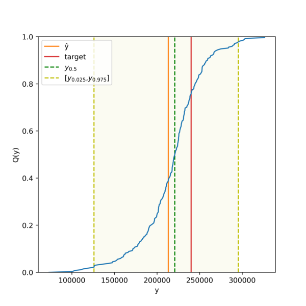
We may request that the predict_cps method returns the full conformal predictive distribution (CPD) for each test instance, as defined by the threshold values, by setting return_cpds=True. The format of the distributions vary with the type of conformal predictive system; for a standard and normalized CPS, the output is an array with a row for each test instance and a column for each calibration instance (residual), while for a Mondrian CPS, the default output is a vector containing one CPD per test instance, since the number of values may vary between categories.

cpds = rf.predict_cps(X_test, sigmas=sigmas_test, bins=bins_test, return_cpds=True)

The resulting vector of arrays is not displayed here, but we instead provide a plot for the CPD of a random test instance:

Examples

For additional examples of how to use the package and module, see the documentation, this Jupyter notebook using WrapClassifier and WrapRegressor, and this Jupyter notebook using ConformalClassifier, ConformalRegressor, and ConformalPredictiveSystem.

Citing crepes

If you use crepes for a scientific publication, you are kindly requested to cite the following paper:

Boström, H., 2022. crepes: a Python Package for Generating Conformal Regressors and Predictive Systems. In Conformal and Probabilistic Prediction and Applications. PMLR, 179. Link

Bibtex entry:

@InProceedings{crepes,
  title = 	 {crepes: a Python Package for Generating Conformal Regressors and Predictive Systems},
  author =       {Bostr\"om, Henrik},
  booktitle = 	 {Proceedings of the Eleventh Symposium on Conformal and Probabilistic Prediction and Applications},
  year = 	 {2022},
  editor = 	 {Johansson, Ulf and Boström, Henrik and An Nguyen, Khuong and Luo, Zhiyuan and Carlsson, Lars},
  volume = 	 {179},
  series = 	 {Proceedings of Machine Learning Research},
  publisher =    {PMLR}
}

References

[1] Vovk, V., Gammerman, A. and Shafer, G., 2005. Algorithmic learning in a random world. Springer Link

[2] Papadopoulos, H., Proedrou, K., Vovk, V. and Gammerman, A., 2002. Inductive confidence machines for regression. European Conference on Machine Learning, pp. 345-356. Link

[3] Johansson, U., Boström, H., Löfström, T. and Linusson, H., 2014. Regression conformal prediction with random forests. Machine learning, 97(1-2), pp. 155-176. Link

[4] Boström, H., Linusson, H., Löfström, T. and Johansson, U., 2017. Accelerating difficulty estimation for conformal regression forests. Annals of Mathematics and Artificial Intelligence, 81(1-2), pp.125-144. Link

[5] Boström, H. and Johansson, U., 2020. Mondrian conformal regressors. In Conformal and Probabilistic Prediction and Applications. PMLR, 128, pp. 114-133. Link

[6] Vovk, V., Petej, I., Nouretdinov, I., Manokhin, V. and Gammerman, A., 2020. Computationally efficient versions of conformal predictive distributions. Neurocomputing, 397, pp.292-308. Link

[7] Boström, H., Johansson, U. and Löfström, T., 2021. Mondrian conformal predictive distributions. In Conformal and Probabilistic Prediction and Applications. PMLR, 152, pp. 24-38. Link

[8] Vovk, V., 2022. Universal predictive systems. Pattern Recognition. 126: pp. 108536 Link

---

Author: Henrik Boström ([e-mail]) Copyright 2023 Henrik Boström License: BSD 3 clause

References

[1] Vovk, V., Gammerman, A. and Shafer, G., 2022. Algorithmic learning in a random world. 2nd edition. Springer Link