Structural heterogeneous cryoEM reconstruction: https://github.com/Gabriel-Ducrocq/cryoSPHERE

Project description
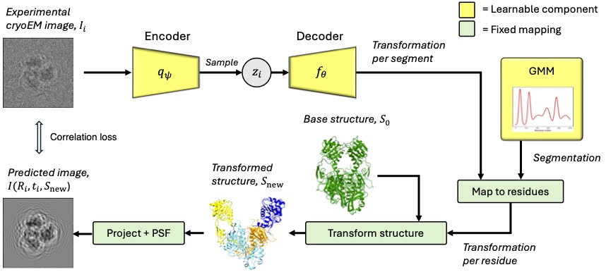
cryoSPHERE: Single-particle heterogeneous reconstruction from cryo EM
CryoSPHERE is a structural heterogeneous reconstruction software of cryoEM data. It requires an estimate of the CTF and poses of each image. This can be obtained using other softwares.
CryoSPHERE works with two yaml files: one parameters.yaml describing the hyperparameters used to train cryoSPHERE and a image.yaml file, describing the images in the dataset. You can find a commented example of these files in the repository.
The file parameters.yaml describes how to fit a single segmentation for the entire protein.
The file parameters_two_segmentation.yaml describes how you can segment chain A and chain C (for example) only, and how to create a custom starting segmentation and define a custom prior on the segmentation. Note that if these custom starting segmentation and prior are not defined, the values of the segmentation are taken so that it is uniform. See the class Segmentation in the file segmentation.py.
Installation
CryoSPHERE is available as a python package named cryosphere. Create a conda environment, install cryosphere with pip and then pytorch3d:
conda create -n cryosphere python==3.9.20
conda activate cryosphere
conda install pytorch3d -c pytorch3d -c conda-forge
pip install cryosphere
Training
Preliminary: consensus reconstruction.
Before running cryoSPHERE on a dataset you need to run a homogeneous reconstruction software such as RELION or cryoSparc. This should yield a star file containing the poses of each image, the CTF and information about the images as well as one or several mrcs file(s) containing the actual images. You should also obtain one or several mrc files corresponding to consensus reconstruction(s). For this tutorial, we assume your images are in a file called particles.mrcs and after a consensus reconstruction, you obain a star file named particles.star and a consensus reconstruction file called consensus_map.mrc. This naming is not mandatory, your files can have arbitrary names as long as the extension is correct. CryoSPHERE would also work with data preprocessed by cryoSparc. In that case you can directly use the particles.cs file.
This step is important to obtain an estimation of the CTF and the pose of each image.
First step: centering the structure
Fit a good atomic structure of the protein of interest into the volume obtained in the prelimiary step (consensus_map.mrc), using e.g ChimeraX. Save this structure in pdb format: fitted_structure.pdb. You can now use cryoSPHERE's command line tools to center the structure and volume:
cryosphere_center_origin --pdb_file_path fitted_structure.pdb --mrc_file_path consensus_map.mrc
This yields a pdb file fitted_structure_centered.pdb of the centered structure and a mrc file consensus_map_centered.mrc of the centered consensus volume.
First step bis (optional)
Since the datasets are usually very noisy, it might be helpful to apply a low pass filter to the images. To determine the bandwith cutoff, first turn the centered structure into a volume, using the same GMM representation of the protein used during the training of cryoSPHERE:
cryosphere_structure_to_volume --image_yaml /path/to/image.yaml --structure_path/path/to/fitted_structure_centered.pdb --output_path /path/to/fitted_structure_centered_volume.mrc
You can now compute the Fourier Shell Correlation (FSC) between fitted_structure_centered_volume.mrc and consensus_map_centered.mrc using available softwares: e.g the e2proc3d command of EMAN2 or online here.
Next, find the frequency cutoff_freq for which the FSC is equal to 0.5, and set lp_bandwidth: 1/cutoff_freq in the parameters.yaml. This means that the in the images, the frequencies such that freq > 1/lp_bandwidth are set to 0.
Second step
The second step is to run cryoSPHERE. To run it, you need two yaml files: a parameters.yaml file, defining all the parameters of the training run and a image.yaml file, containing informations about the images. You need to set the folder_experiment entry of the paramters.yaml to the path of the folder containing your data. You also need to change the base_structure entry to fitted_structure_centered.pdb. You can then run cryosphere using the command line tool:
cryosphere_train --experiment_yaml /path/to/parameters.yaml
This command creates a folder named cryoSPHERE which contains the PyTorch models ckpt_{n_epoch}.pt and the segmentations seg_{n_epoch}.pt, one at the end of each epoch. It also copies the parameters.yaml and image.yaml files in this directory and creates a run.log to log training data.
You can customize the parameters.yaml file, especially the segmentation. You can choose between a global segmentation of the protein and a local one.
The global segmentation is demonstrated in parameters.yaml and only requires you to set the number of segments and the entry all_protein: True. Be careful that this segmentation considers the entire protein as a single chain, where the residues are ordered as in the pdb file of the base structure you are using.
The local segmentation allows you to specify what part of the protein you want to segment, and what part of the protein you want to fix. If your protein has chains e.g A, B, C and D, you can segment only the residues 0 to 50 of chain A and the residues 130 to 240 of chain C. The remaining residues of the protein will not move. These two segmentations are "separate". See parameters_two_segmentation.yaml.
Finally, if you do not specify a starting segmentation, the means of the Gaussian modes of the segmentation are taken evenly along the residues, the standard deviations are all equal to N_residues/N_segmentsand the mean of the porportions are set to 0.
The same is true for the prior distribution on the segmentation. You can specify a starting segmentation or a prior, or both, or none, for each part you are segmenting. See parameters_two_segmentation.yaml for an example.
Analysis
Once cryoSPHERE has been trained, you can get the latent variables corresponding to the images and generate a PCA analysis of the latent space, with latent traversal of first principal components:
cryosphere_analyze --experiment_yaml /path/to/parameters.yaml --model /path/to/model.pt --segmenter /path/to/segmenter.pt --output_path /path/to/outpout_folder --no-generate_structures
where model.pt is the saved torch model you want to analyze, segmenter.pt is the corresponding segmentation and output_folder is the folder where you want to save the results of the analysis.
This will create the following directory structure:
analysis
   |	z.npy
   |	pc0
	   |   structure_z_1.pdb
	   .
	   .
	   .
	   |   structure_z_10.pdb
           |    pca.png

   |	pc1
	   |   structure_z_1.pdb
	   .
	   .
           .
If you want to generate all structures (one for each image), you can set --generate_structures instead. This will skip the PCA step. The file z.npy contains the latent variable associated to each image (in the same order as the images in the star file), the .pdb files are the structures sampled along the principal component (from lowest to highest values along that PC) and the .png files are images of the PCA decompositions.
It is also possible to get the structures corresponding to specific images. Save the latent variables corresponding to the images of interest into a z_interest.npy. You can then run:
cryosphere_analyze --experiment_yaml /path/to/parameters.yaml --model /path/to/model.pt --output_path /path/to/outpout_folder --z /path/to/z_interest.npy --segmenter /path/to/segmenter.pt --generate_structures
Setting the --z /path/to/z_interest.npy argument will directly decode the latent variables in z_interest.npy into structures.
Release history Release notifications | RSS feed


Download files
Download the file for your platform. If you're not sure which to choose, learn more about installing packages.
Source Distribution
Built Distribution
Filter files by name, interpreter, ABI, and platform.
If you're not sure about the file name format, learn more about wheel file names.
Copy a direct link to the current filters
File details
Details for the file cryosphere-0.4.6.tar.gz.
File metadata
- Download URL: cryosphere-0.4.6.tar.gz
- Upload date:
- Size: 125.7 kB
- Tags: Source
- Uploaded using Trusted Publishing? No
- Uploaded via: twine/6.1.0 CPython/3.10.4
File hashes
| Algorithm | Hash digest | |
|---|---|---|
| SHA256 |
bd7cda29a080664d4380ed0d691a464fef930c5affddd5bb38f18e4115687355
|
|
| MD5 |
ab2adc9eaed252b9686263e4ba8c56d9
|
|
| BLAKE2b-256 |
d4145a95ed4772f88d5f59639e14547296be306a9f443820a51d66c28c67ce64
|
File details
Details for the file cryosphere-0.4.6-py3-none-any.whl.
File metadata
- Download URL: cryosphere-0.4.6-py3-none-any.whl
- Upload date:
- Size: 128.2 kB
- Tags: Python 3
- Uploaded using Trusted Publishing? No
- Uploaded via: twine/6.1.0 CPython/3.10.4
File hashes
| Algorithm | Hash digest | |
|---|---|---|
| SHA256 |
0d328885bdda34bffd369564f6e2529ff4f201c60a649192e4d5bb5e052bf772
|
|
| MD5 |
310b437bb609a06068285db83ab0bc83
|
|
| BLAKE2b-256 |
828ec67eb7c1190a34211dee302bbd3bc0ec621ac972090e800d03c66587bc98
|


