Cryogenic thermal calculations library for cryostat design

Project description
CryoHeatFlow
A Python package for cryogenic thermal analysis and heat transfer calculations. This package provides functions for calculating thermal conductivity, thermal power transfer, thermal boundary conductance, and multilayer insulation effectiveness.
Installation
pip install cryoheatflow
Table of Contents
Features
- Thermal conductivity calculations for various materials at cryogenic temperatures
- Thermal power transfer through conductors and insulators
- Thermal boundary conductance across joints and interfaces
- Multilayer insulation effectiveness calculations
- Area calculations for various cross-sectional geometries
Quick Start
Calculate Thermal Conductivity
import cryoheatflow

# Get thermal conductivity for stainless steel at 10K
k_conductivity_function = cryoheatflow.conductivity.k_ss
T = 10  # Temperature in Kelvin
result = k_conductivity_function(T)
print(f'Thermal conductivity = {result} W/m*K')
Calculate Thermal Power Transfer
Let's say you wanted to connect a stainless-steel microwave coax line from a 40K stage to a 4K stage. The coax has a diameter of 0.085" (so-called "085" coax), and is 30mm long. How much heat would be transferred?
import cryoheatflow

# Select stainless steel as the material
k = cryoheatflow.conductivity.k_ss
area = cryoheatflow.area.coax_085  # 0.085" outer-diameter coax
length = 30e-3  # 30 mm
T1 = 40  # 40 K
T2 = 4   # 4 K

P, G, R = cryoheatflow.calculate_thermal_transfer(k, area, length, T1, T2)
print(f'Power transmission = {P*1e3:0.3f} mW')
print(f'Thermal conductance = {G:0.6f} W/K')
print(f'Thermal resistance = {R:0.3f} K/W')
giving us
Power transmission = 4.844 mW
Thermal conductance = 0.000135 W/K
Thermal resistance = 7432.015 K/W
Calculate thermal boundary conductance
Now let's say you want to anchor a 1.5x1.5 cm^2 sample to your 4K stage, and you put grease between the sample and the 4K stage. Your sample is going to generate 2 mW of heat load and going to warm up a little. What temperature is your sample going to be at?
First, we calculate the thermal boundary conductance (in watts per kelvin), and/or its inverse quantity, the thermal boundary resistance:
import cryoheatflow

# Calculate thermal boundary conductance across a solder joint
T = 4  # Temperature in Kelvin
area_m2 = 15e-3 * 15e-3  # 15 mm x 15 mm contact area

h = cryoheatflow.conductivity.h_grease(T=T, area=area_m2)
print(f'Thermal conductance = {h:0.3f} W/K')
print(f'Thermal resistance = {1/h:0.3f} K/W')
This gives us Thermal resistance R = 38.384 K/W. We can then estimate the temperature by the simple relation
(temperature increase) = (thermal resistance) x (heating power)
Giving us a temperature increase of ~76.8 mK.
Multilayer Insulation Analysis
from cryoheatflow import solve_multilayer_insulation
from cryoheatflow.emissivity import Al_polished, Al_oxidized, mylar

# Calculate effectiveness of multilayer insulation
T1 = 4   # Cold side temperature (K)
T2 = 85  # Warm side temperature (K)
N = 2    # Number of mylar layers
emissivity1 = Al_oxidized    # Emissivity of the first layer (e.g. 300K walls)
emissivity_mylar = mylar     # Emissivity of the multilayer mylar layers
emissivity2 = Al_polished    # Emissivity of the last layer (e.g. 40K walls)
area = (20e-2)**2           # Area in m^2

layer_temps, qdot = solve_multilayer_insulation(T1, T2, N, emissivity1, emissivity_mylar, emissivity2, area)
print(f'Layer temperatures: {layer_temps}')
print(f'Thermal power: {abs(qdot)} W')
Plotting Thermal Conductivity Curves
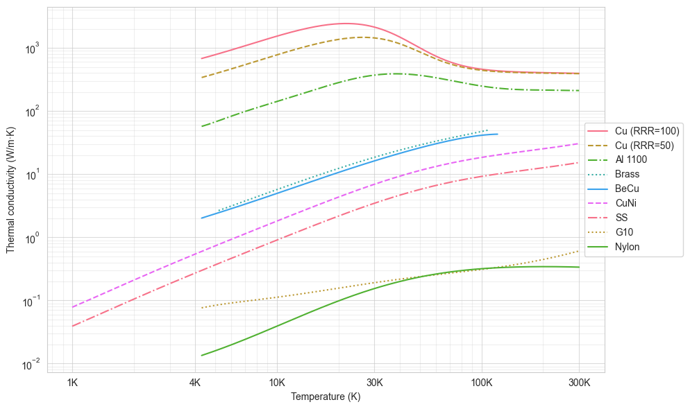
from cryoheatflow.conductivity import ( k_ss, k_cuni, k_al6061, k_al6063, k_brass,
     k_cu_rrr50, k_al1100, k_becu, k_cu_rrr100, k_g10, k_nylon)
import matplotlib.pyplot as plt
import numpy as np

# Plot thermal conductivity vs temperature for all materials
k_funcs = [k_ss, k_cuni, k_al6061, k_al6063, k_al1100, k_becu, k_brass,
           k_cu_rrr50, k_cu_rrr100, k_g10, k_nylon]

labels = ['SS', 'CuNi', 'Al 6061-T6', 'Al 6063-T5', 'Al 1100',
          'BeCu', 'Brass', 'Cu (RRR=50)', 'Cu (RRR=100)', 'G10', 'Nylon']
for k_fun in k_funcs:
    T = np.linspace(4, 300, 1000)
    k = k_fun(T)
    plt.loglog(T, k)

plt.xlabel('Temperature (K)')
plt.ylabel('Thermal conductivity (W/m*K)')
plt.legend(labels, loc='lower right')
plt.show()
Available Materials
Thermal Conductivity Functions
The package provides thermal conductivity functions for various materials from the NIST cryogenic thermal conductivity reference:
k_ss- Stainless steel (316/314/304L)k_cuni- 70-30 CuNi cupronickelk_al6061- Aluminum 6061-T6k_al6063- Aluminum 6063-T5k_al1100- Aluminum 1100k_brass- Brass (UNS C26000)k_becu- Beryllium copperk_cu_rrr50- Copper (RRR=50, typically ETP or OFHC)k_cu_rrr100- Copper (RRR=100)k_g10- Fiberglass-epoxy (G-10)k_nylon- Nylon (polyamide)
Thermal Boundary Conductance Functions
h_grease- Thermal conductance of grease for given contact areah_solder_pb_sn- Thermal conductance of standard lead-tin (PbSn) solder for given contact area
Emissivity Values
Al_polished- Polished aluminum (ε = 0.03)Al_oxidized- Oxidized aluminum (ε = 0.3)Cu_polished- Polished copper (ε = 0.02)Cu_oxidized- Oxidized copper (ε = 0.6)brass_polished- Polished brass (ε = 0.03)brass_oxidized- Oxidized brass (ε = 0.6)stainless- Stainless steel (ε = 0.07)mylar- Mylar (ε = 0.05)
Area Calculations
The package includes functions for calculating cross-sectional areas:
tube_area(diameter, wall_thickness)- Annular cross-section areacylinder_area(diameter)- Circular cross-section areawire_gauge_area(awg)- Wire cross-section area based on AWG gaugecoax_141,coax_085,coax_047,coax_034- Predefined coaxial cable areas
Data Sources
Thermal conductivity data is sourced from the NIST Cryogenics Materials Database: https://trc.nist.gov/cryogenics/materials/materialproperties.htm
Emissivity and thermal boundary conductance values are from Ekin, J. (2006), Experimental Techniques for Low-Temperature Measurements, Oxford University Press, Oxford, UK.
Requirements
- Python >= 3
- NumPy
- SciPy
- Matplotlib (for plotting examples)
Release history Release notifications | RSS feed


Download files
Download the file for your platform. If you're not sure which to choose, learn more about installing packages.
Source Distribution
Built Distribution
Filter files by name, interpreter, ABI, and platform.
If you're not sure about the file name format, learn more about wheel file names.
Copy a direct link to the current filters
File details
Details for the file cryoheatflow-0.9.0.tar.gz.
File metadata
- Download URL: cryoheatflow-0.9.0.tar.gz
- Upload date:
- Size: 19.7 kB
- Tags: Source
- Uploaded using Trusted Publishing? No
- Uploaded via: twine/6.1.0 CPython/3.11.3
File hashes
| Algorithm | Hash digest | |
|---|---|---|
| SHA256 |
27fc99789c9393f65e27fa4c2b0200610a0df0d9a36e4a9f6d55cec558d981f7
|
|
| MD5 |
d2a9facf8710ede03dc5b4556a3ec293
|
|
| BLAKE2b-256 |
278f21fe74b0a8122be9b9fcc9321da2ceec39537d9091e9c52a391131d1b5ad
|
File details
Details for the file cryoheatflow-0.9.0-py3-none-any.whl.
File metadata
- Download URL: cryoheatflow-0.9.0-py3-none-any.whl
- Upload date:
- Size: 20.6 kB
- Tags: Python 3
- Uploaded using Trusted Publishing? No
- Uploaded via: twine/6.1.0 CPython/3.11.3
File hashes
| Algorithm | Hash digest | |
|---|---|---|
| SHA256 |
15b9c18bedc9dd92c45c099a02f37f625b325057c04ae174a8a9f6cea59818bb
|
|
| MD5 |
4523122709139d8e841f83316549336a
|
|
| BLAKE2b-256 |
e62eb3484e3f98b9be52cdacd4e659a5022fd200b7762e64a46022a7f7d29b4f
|


