csfpy 0.1.9.3

An Analytical Engine for Non-Prismatic Structural Members

Continuous Section Field (CSF)

A Python framework for axially graded non-uniform structural members

Key Features • Installation & setup • Worked Example • Validation: Cylinder • Case Study: NREL 5-MW

---

📚 CSF Building Blocks Fundamentals - CSF Geometry, Sections, Polygon Tags, and Weight Laws Guide.

---

Motivation

CSF provides a continuous representation of the variable geometry and material distribution of non-prismatic members along the longitudinal coordinate (z). Geometric and mechanical variations are defined directly as continuous fields rather than through a sequence of discrete member segments.

It represents the variable geometry and material distribution as continuous functions of $z$, computing the resulting properties - $A(z)$, $I_x(z)$, $I_y(z)$, together with the associated material details along the member. The resulting data can be exported in CSV and YAML formats for integration with beam solvers such as OpenSees and SAP2000, or with section-analysis tools such as csf_sp and sp_csf.

---

Three-dimensional representation of the tapered pole with localized degradation. Gray regions indicate the non-degraded portions.

Full reproducible example: Tapered prestressed degraded concrete pole

---

CSF combines:

• Geometry field: arbitrary polygonal sections defined at stations (S0, S1) with continuous interpolation for tapered or varying shapes.

• Axial/bending weight field: per-polygon participation factor w_i(z) along the longitudinal axis, scaling each region’s effective contribution to area, axial, and bending-related section properties.

• Shear/torsion weight field: per-polygon participation factor shear_w_i(z) along the longitudinal axis, allowing shear/torsion-related contributions to vary independently from w_i(z).

  See Ekofisk Jacket Platform - Foundation Piles for a localized corrosion case.

---

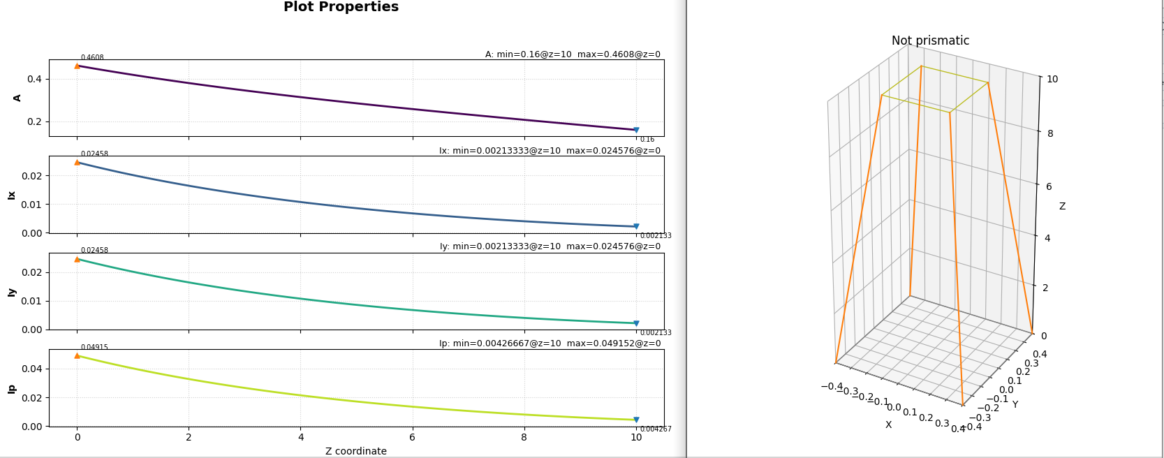
CSF accepts two input files: geometry.yaml (cross-section definition) and actions.yaml (post-processing pipeline).

geometry.yaml file

# geometry.yaml
# Defines the cross-sectional geometry and material participation laws
# of the structural member.
#
# - sections: end cross-sections (S0, S1) with polygon vertices at each
#   z-station.
# - polygons: 2D closed polygons, defined by ordered vertices, that compose
#   each cross-section.
# - vertices: polygon coordinates in the local section plane; vertices should
#   be given in counter-clockwise (CCW) order for positive area.
# - weight: base participation factor assigned to each polygon.
# - weight_laws: longitudinal participation laws w(z) that scale each polygon's
#   contribution along the member axis, independently of geometric interpolation.
# - shear_weight_laws: longitudinal shear/torsional participation laws shear_w(z),
#   used to scale shear- and torsion, related contributions independently from w(z).
# - iso(nu): isotropic shortcut that derives shear participation from weight
#   using G = E / [2 * (1 + nu)].

CSF:
  sections:
    S0:
      z: 0.0
      polygons:
        startsection:
          weight: 1.0
          vertices:
            - [-0.4, -0.4]
            - [0.4, -0.4]
            - [0.4, 0.4]
            - [-0.4, 0.4]
    S1:
      z: 10.0
      polygons:
        endsection:
          weight: 1.0
          vertices:
            - [-0.2, -0.2]
            - [0.2, -0.2]
            - [0.2, 0.2]
            - [-0.2, 0.2]
  # shear_weight_laws: longitudinal shear participation laws shear_w(z),
  # used to scale torsion/shear-related contributions independently from w(z)
  shear_weight_laws:
  # isotropic shortcut: sets shear_w(z) from w(z) using G = E / [2 * (1 + nu)]
  - 'startsection,endsection: iso(0.2)'
  weight_laws:
  # parabolic increase: 72% at base (z=0), full section at top (z=10)
  - 'startsection,endsection:1.0 - 0.28 * (1 - (z / 10.0)**2)'                 

actions.yaml file

# actions.yaml
# Defines the post-processing operations to run on the CSF model.
# - stations: named z-coordinate sets used as analysis points
# - actions: ordered list of operations (3D plots, section analysis, property export, etc.)

CSF_ACTIONS:
  stations:
    station_edge:
      - 0
      - 10
  actions:  
    - plot_volume_3d:
        params:
          title: "Not prismatic"          
    - plot_weight:
        output:
          - stdout
    - plot_properties:
        properties: [A,Ix,Iy,Ip]
    - plot_section_2d:
        stations:
          - station_edge
    - section_selected_analysis:
        stations:
          - station_edge
        properties: [A, Cx, Cy, Ix, Iy, Ixy, Ip, I1, I2, rx, ry, Wx, Wy,J_s_vroark, J_s_vroark_fidelity]
    - volume:
        stations:
          - station_edge
        output:
          - stdout
          - volume_report.txt
                                   

then run

linux / Mac

python3 -m venv venv
source venv/bin/activate
pip install csfpy
csf-actions geometry.yaml actions.yaml

Windows

py install 3.12
py -V:3.12 -m venv venv
.\venv\Scripts\activate
pip install csfpy
csf-actions geometry.yaml actions.yaml

Minimal working CSF model: two sections, one polygon per section, custom weight laws, isotropic shear_weight_laws, and automatic evaluation of continuous section properties along the member axis.

---

CSF Geometry, Sections, Polygon Tags, and Weight Laws Guide

Example list Complete worked example covering all available actions on a tapered rectangular section

---

Using CSF as a Python Library

CSF is not only a command-line tool, but also a Python library

It can be imported and used programmatically to define geometries, evaluate section properties along the longitudinal axis, and integrate with custom workflows or external solvers.

Full Python API example - Tapered T-beam

---

Key Features

• Polygon-based section representation (algebraic composition): The element is geometrically defined by its end cross-sections, each represented as an algebraic composition of 2D polygons; intermediate sections are generated from these definitions along z. Curved outlines (e.g., circular shells/towers) are represented through discretized polygons with user-selected vertex count.

• Per-polygon longitudinal weight laws $w_i(z)$: property contributions can vary along the member axis independently of geometric interpolation. Weight laws can be defined analytically or via lookup-based expressions.

  • Weight expressions have access to w0, w1 (weights at sections s0/s1) and distance functions d(i,j), di(i,j), de(i,j) between polygon points. Custom Weight Laws

Section vertices can be generated from any CAD tool or script that can sample points along a curve and export their coordinates.

Geometric scope and limitations
CSF is not a FEM solver: it provides a geometric formulation for non-prismatic members and returns sectional properties (and derived stiffness fields) for beam-based analysis or external solvers.
Curved outlines are handled by polygonal approximation (increase the number of sides to reach the desired accuracy).

---

CSFStacked module (segmented ContinuousSectionField stacking)

CSFStacked is a container that stacks multiple ContinuousSectionField segments along the global z axis and dispatches any query z -> correct segment.
It adds a practical layer on top of multiple CSF segments: junctions are handled deterministically and you can query sections/properties anywhere with a single global API (section(z), section_full_analysis(z))

---

🛠 Installation

Linux / Mac

Option A - Install from PyPI (recommended)

python3 -m venv venv
source venv/bin/activate
pip install csfpy

 # you need both geometry.yaml and actions.yaml files
csf-actions geometry.yaml actions.yaml

Option B - Local editable install (development)

python3 -m venv venv
source venv/bin/activate
git clone https://github.com/giovanniboscu/continuous-section-field.git
cd continuous-section-field
pip install -e .

python3 example/nrel_5mw_tower.py
python3 example/cylinder_withcheck.py
python3 example/csf_rotated_validation_benchmark.py

cd actions-examples/stell_degradated_model
mkdir -p out
csf-actions stell_degradated_model_s.yaml stell_degradated_model_action.yaml

---

Windows

py install 3.12

Option 1 - Install from PyPI (recommended)

py install 3.12
py -3.12 -m venv venv
.\venv\Scripts\activate
pip install csfpy

 # you need both geometry.yaml and actions.yaml files
csf-actions geometry.yaml actions.yaml

Option 2 - Local editable install (development)

py install 3.12
py -3.12 -m venv venv
.\venv\Scripts\activate
git clone https://github.com/giovanniboscu/continuous-section-field.git
cd continuous-section-field
pip install -e .

python .\example\nrel_5mw_tower.py
python .\example\cylinder_withcheck.py
python .\example\csf_rotated_validation_benchmark.py
python .\example\tsection_lab.py

cd actions-examples\stell_degradated_model
csf-actions stell_degradated_model_s.yaml stell_degradated_model_action.yaml

---

Cross-sectional properties

At each longitudinal station, CSF evaluates the polygonal zones that define the cross-section and computes the contribution of each zone to the requested sectional property. The final value is obtained by accumulating the zone-wise geometric contributions after applying the corresponding participation field. Geometry and participation therefore remain distinct: the polygon defines the occupied region, while the participation field controls the effective contribution of that region to the sectional property.

CSF – Section Full Analysis Output

---

CSF Numerical Validation: Circular Hollow Section

examples/cylinder_withcheck.py

To verify the accuracy of the numerical engine, a validation test was performed using a non-tapered hollow cylinder (steel pipe). This allows for a direct comparison between the library's results (based on weighted polygons) and exact analytical formulas.

The test script cylinder_withcheck.py models a tower with a diameter of 4.935m and a thickness of 23mm using a 512-sided polygon. The results demonstrate that the polygonal approximation converges to the analytical solution with exceptional precision.

Extended Validation Report

The following table reports the full output of the validation script, comparing Theoretical (Analytical) values with the Numerical results generated by the library.

Structural Property	Sym	Theoretical	Numerical	Error	Unit
Net material cross-section	A	3.54924572e-01	3.54915663e-01	0.0025%	m²
Horizontal center of mass	Cx	0.00000000e+00	5.44816314e-15	5.45e-15 (abs)	m
Vertical center of mass	Cy	0.00000000e+00	-4.12383916e-14	4.12e-14 (abs)	m
Axial stiffness	EA	7.45341600e+10	7.45322893e+10	0.0025%	N
Bending stiffness about X	EIxx	2.24797570e+11	2.24786286e+11	0.0050%	N·m²
Bending stiffness about Y	EIyy	2.24797570e+11	2.24786286e+11	0.0050%	N·m²
Symmetry check (Ixy)	Ixy	0.00000000e+00	3.45889405e-15	3.46e-15 (abs)	m⁴
Torsional stiffness constant	J	2.14092924e+00	2.14082177e+00	0.0050%	m⁴
Torsional stiffness (GJ)	GJ	1.72987083e+11	1.72978399e+11	0.0050%	N·m²
Maximum bending stiffness	EI_max	2.24797570e+11	2.24786286e+11	0.0050%	N·m²
Minimum bending stiffness	EI_min	2.24797570e+11	2.24786286e+11	0.0050%	N·m²
Principal axis rotation	Alpha	0.00000000e+00	0.00000000e+00	0.0000% (Iso)	deg
Buckling radius about X	rx	1.73667329e+00	1.73665150e+00	0.0013%	m
Buckling radius about Y	ry	1.73667329e+00	1.73665150e+00	0.0013%	m
First moment of area (Shear)	Q	2.77471084e-01	2.77460637e-01	0.0038%	m³
Elastic Section Modulus	W	4.33825580e-01	4.33803803e-01	0.0050%	m³
Mass per unit length	m_lin	2.78615789e+03	2.78608796e+03	0.0025%	kg/m

Total Calculated Tower Volume: 31.041 m³
Total Calculated Tower Mass: 243.676 t

Description	Theoretical	Numerical	Error	Unit
Total Tower Mass	244.067	244.061	0.0025%	t

CSF Validation : Numerical Case Study: NREL 5-MW Reference Wind Turbine Tower

CSF is listed as a third-party tool in the OpenFAST documentation

• NREL 5-MW reference turbine report: Jonkman, J., Butterfield, S., Musial, W., and Scott, G.
  "Definition of a 5-MW Reference Wind Turbine for Offshore System Development,"
  NREL/TP-500-38060, February 2009.
  • Download PDF (NREL)
  • OpenFAST documentation
  • NLR wind research portal

512sided polygons

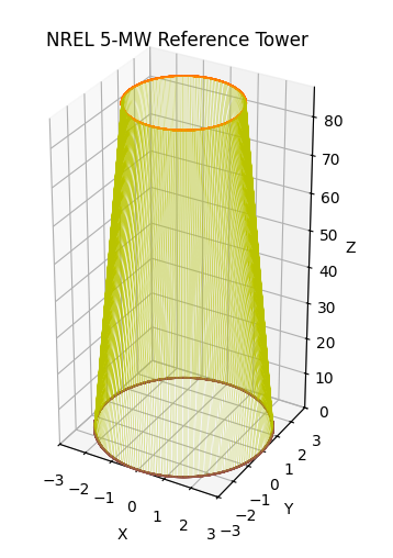
CSF computes continuous sectional properties along the tower height (z) - (A(z)), (EI(z)), (GJ(z)), etc. - compatible with OpenFAST ElastoDyn/SubDyn distributed property requirements and validated against NREL 5‑MW reference data.

The script example/nrel_5mw_tower.py is used to demonstrate the library's performance on complex, real-world structural members. A full-scale model of the NREL 5-MW Reference Wind Turbine Tower was implemented. The geometry and material properties strictly follow the technical report "Definition of a 5-MW Reference Wind Turbine for Offshore System Development" (NREL/TP-500-38060).

The following tables provide a side-by-side comparison between the Numerical results generated by CSF and the official NREL reference data (Table 6-1 of the official PDF).

Density = 8500 kg/m3

CSF Numerical Results (Generated Model)

Elevation [m]	HtFract	TMassDen [kg/m]	TwFAStif [N·m²]	TwSSStif [N·m²]	TwGJStif [N·m²]	TwEAStif [N]	TwFAIner [kg·m]	TwSSIner [kg·m]
0.00	0.000	5590.73	6.1431e+11	6.1431e+11	4.7273e+11	1.3812e+11	2.49e+04	2.49e+04
8.76	0.100	5232.30	5.3479e+11	5.3479e+11	4.1154e+11	1.2927e+11	2.16e+04	2.16e+04
17.52	0.200	4885.64	4.6324e+11	4.6324e+11	3.5648e+11	1.2070e+11	1.88e+04	1.88e+04
26.28	0.300	4550.76	3.9911e+11	3.9911e+11	3.0713e+11	1.1243e+11	1.62e+04	1.62e+04
35.04	0.400	4227.65	3.4187e+11	3.4187e+11	2.6307e+11	1.0445e+11	1.38e+04	1.38e+04
43.80	0.500	3916.31	2.9100e+11	2.9100e+11	2.2393e+11	9.6756e+10	1.18e+04	1.18e+04
52.56	0.600	3616.74	2.4601e+11	2.4601e+11	1.8931e+11	8.9355e+10	9.96e+03	9.96e+03
61.32	0.700	3328.95	2.0645e+11	2.0645e+11	1.5887e+11	8.2245e+10	8.36e+03	8.36e+03
70.08	0.800	3052.93	1.7184e+11	1.7184e+11	1.3224e+11	7.5425e+10	6.96e+03	6.96e+03
78.84	0.900	2788.68	1.4177e+11	1.4177e+11	1.0909e+11	6.8897e+10	5.74e+03	5.74e+03
87.60	1.000	2536.21	1.1581e+11	1.1581e+11	8.9122e+10	6.2659e+10	4.69e+03	4.69e+03

Total Calculated Tower Volume: 40.8634 m³
Total Calculated Tower Mass: 347.339 t
 

Official NREL 5-MW Tower Data (Reference Table 6-1, p. 15)

Elevation [m]	HtFract	TMassDen [kg/m]	TwFAStif [N·m²]	TwSSStif [N·m²]	TwGJStif [N·m²]	TwEAStif [N]	TwFAIner [kg·m]	TwSSIner [kg·m]
0.00	0.000	5590.9	6.143e+11	6.143e+11	4.728e+11	1.381e+11	2.49e+04	2.49e+04
8.76	0.100	5232.4	5.348e+11	5.348e+11	4.116e+11	1.293e+11	2.16e+04	2.16e+04
17.52	0.200	4885.8	4.633e+11	4.633e+11	3.565e+11	1.207e+11	1.88e+04	1.88e+04
26.28	0.300	4550.9	3.991e+11	3.991e+11	3.071e+11	1.124e+11	1.62e+04	1.62e+04
35.04	0.400	4227.8	3.419e+11	3.419e+11	2.631e+11	1.044e+11	1.38e+04	1.38e+04
43.80	0.500	3916.4	2.910e+11	2.9100e+11	2.239e+11	9.676e+10	1.18e+04	1.18e+04
52.56	0.600	3616.8	2.460e+11	2.460e+11	1.893e+11	8.936e+10	9.96e+03	9.96e+03
61.32	0.700	3329.0	2.065e+11	2.065e+11	1.589e+11	8.225e+10	8.36e+03	8.36e+03
70.08	0.800	3053.0	1.718e+11	1.718e+11	1.322e+11	7.543e+10	6.96e+03	6.96e+03
78.84	0.900	2788.8	1.418e+11	1.418e+11	1.091e+11	6.890e+10	5.74e+03	5.74e+03
87.60	1.000	2536.3	1.158e+11	1.158e+11	8.913e+10	6.266e+10	4.69e+03	4.69e+03

Total NREL 5-MW Ref. Mass: 347.460 t

Relative error (Generated − Reference) / Reference × 100

Elevation [m]	HtFract	TMassDen [kg/m]	TwFAStif [N·m²]	TwSSStif [N·m²]	TwGJStif [N·m²]	TwEAStif [N]	TwFAIner [kg·m]	TwSSIner [kg·m]
0.00%	0.00%	0.0030%	0.0016%	0.0016%	0.0148%	0.0145%	0.00%	0.00%
0.00%	0.00%	0.0019%	0.0019%	0.0019%	0.0146%	0.0232%	0.00%	0.00%
0.00%	0.00%	0.0033%	0.0130%	0.0130%	0.0056%	0.0000%	0.00%	0.00%
0.00%	0.00%	0.0031%	0.0025%	0.0025%	0.0098%	0.0267%	0.00%	0.00%
0.00%	0.00%	0.0035%	0.0088%	0.0088%	0.0114%	0.0479%	0.00%	0.00%
0.00%	0.00%	0.0023%	0.0000%	0.0000%	0.0134%	0.0041%	0.00%	0.00%
0.00%	0.00%	0.0017%	0.0041%	0.0041%	0.0158%	0.0056%	0.00%	0.00%
0.00%	0.00%	0.0015%	0.0242%	0.0242%	0.0189%	0.0061%	0.00%	0.00%
0.00%	0.00%	0.0023%	0.0233%	0.0233%	0.0302%	0.0066%	0.00%	0.00%
0.00%	0.00%	0.0043%	0.0212%	0.0212%	0.0092%	0.0044%	0.00%	0.00%
0.00%	0.00%	0.0035%	0.0086%	0.0086%	0.0090%	0.0016%	0.00%	0.00%

Validation Summary

• All discrepancies are well below 0.05%.
• Differences are attributable to rounding and numerical precision.
• The generated CSF tower properties faithfully reproduce the NREL 5-MW reference.

OpenFAST Integration - CSF API Example

For a complete example of CSF integrated into the OpenFAST aeroelastic simulation framework - from parametric tower geometry through BModes to ElastoDyn - see the

HISTWIN Example

Two NREL/OpenFAST tower examples are provided:

• Code-only example: example/nrel_5mw_tower.py
• Formal AES reproducibility case: docs/aes/nrel_case/README.md

---

Worked Example: Continuously Tapered T-Beam

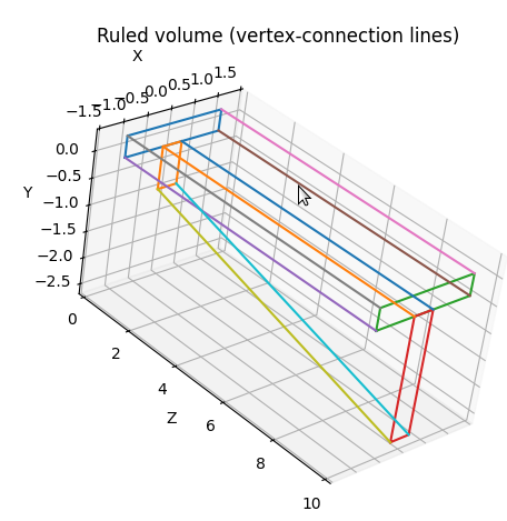
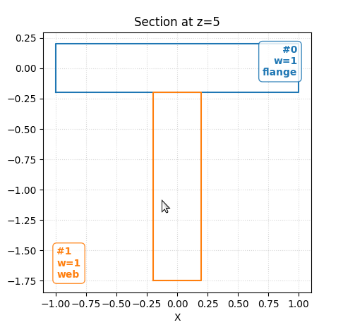
This section demonstrates how to model a structural member where the geometry transitions smoothly between two different T-profiles.

Click to expand the full T-Beam Python example

# --- Core CSF imports used in this minimal example ---
from csf import (
    Pt, Polygon,integrate_volume,section_statical_moment_partial,section_properties, section_derived_properties,Section, ContinuousSectionField,Visualizer,
    section_full_analysis, section_print_analysis,section_full_analysis_keys
)
# ----------------------------------------------------------------------------------
# 1. DEFINE START SECTION (Z = 0)
# ----------------------------------------------------------------------------------
#   GUIDELINES FOR POLYGON CONSTRUCTION:
# - COUNTER-CLOCKWISE POLYGON
# - VERTICES ORDER: You MUST define vertices in COUNTER-CLOCKWISE (CCW) order.
#   This is MANDATORY for the Shoelace/Green's Theorem algorithm to compute a
#   POSITIVE Area and correct Moments of Inertia. Clockwise order will result
#   in negative area values and mathematically incorrect results.
# - WEIGHT: Use 1.0 for solid parts and 0 to define voids/holes.
# - The start section here is a T-shape composed of two non-overlapping polygons:
#   a "flange" (top horizontal) and a "web" (vertical stem).
# ----------------------------------------------------------------------------------

# Flange Definition: Rectangle from (-1, -0.2) to (1, 0.2)
# Order: Bottom-Left -> Bottom-Right -> Top-Right -> Top-Left (CCW)
poly0_start = Polygon(
    vertices=(Pt(-1, -0.2), Pt(1, -0.2), Pt(1, 0.2), Pt(-1, 0.2)),
    weight=1.0,
    name="flange",
)

# Web Definition: Rectangle from (-0.2, -1.0) to (0.2, 0.2)
# Order: Bottom-Left -> Bottom-Right -> Top-Right -> Top-Left (CCW)
poly1_start = Polygon(
    vertices=(Pt(-0.2, -1.0), Pt(0.2, -1.0), Pt(0.2, -0.2), Pt(-0.2, -0.2)),
    weight=1.0,
    name="web",
)

# ----------------------------------------------------------------------------------
# 2. DEFINE END SECTION (Z = 10)
# ----------------------------------------------------------------------------------
# GEOMETRIC CONSISTENCY:
# - To enable linear interpolation (tapering), the end section must contain the
#   same number of polygons with the same names as the start section.
# - The web depth here increases linearly from 1.0 down to 2.5 (negative Y direction),
#   creating a tapered profile along the longitudinal Z-axis.
# ----------------------------------------------------------------------------------

# Flange remains unchanged for this prismatic top part
poly0_end = Polygon(
    vertices=(Pt(-1, -0.2), Pt(1, -0.2), Pt(1, 0.2), Pt(-1, 0.2)),
    weight=1.0,
    name="flange",
)

# Web becomes deeper: Y-bottom moves from -1.0 to -2.5
# MAINTAIN CCW ORDER: Bottom-Left -> Bottom-Right -> Top-Right -> Top-Left
poly1_end = Polygon(
    vertices=(Pt(-0.2, -2.5), Pt(0.2, -2.5), Pt(0.2, -0.2), Pt(-0.2, -0.2)),
    weight=1.0,
    name="web",
)

# ----------------------------------------------------------------------------------
# 3. CREATE SECTIONS WITH Z-COORDINATES
# ----------------------------------------------------------------------------------
# Sections act as containers for polygons at a specific coordinate along the beam axis.
# All polygons defined at Z=0.0 are grouped into s0, and those at Z=10.0 into s1.
# ----------------------------------------------------------------------------------

# Order matters: poly0_start pairs with poly0_end,
# and poly1_start pairs with poly1_end
# because they appear in the same position in their respective sections.

s0 = Section(polygons=(poly0_start, poly1_start), z=0.0)
s1 = Section(polygons=(poly0_end, poly1_end), z=10.0)

# --------------------------------------------------------
# 4. INITIALIZE CONTINUOUS SECTION FIELD
# --------------------------------------------------------
# A linear interpolator is used to generate intermediate
# sections between Z = 0 and Z = 10.
field = ContinuousSectionField(section0=s0, section1=s1)

# --------------------------------------------------------
# 5. PRIMARY SECTION PROPERTIES (Z = 5.0)
# --------------------------------------------------------
# Properties are computed at mid-span.
sec_mid = field.section(5.0)
props = section_properties(sec_mid)

print("\n" + "="*40)
print("PRIMARY PROPERTIES AT Z=5.0 (Centroidal)")
print("="*40)
print(f"A:   {props['A']:.4f}      # Net Cross-Sectional Area")
print(f"Cx:  {props['Cx']:.4f}     # Horizontal Centroid location (Global X)")
print(f"Cy:  {props['Cy']:.4f}     # Vertical Centroid location (Global Y)")
print(f"Ix:  {props['Ix']:.4f}     # Second Moment of Area about Centroidal X-axis")
print(f"Iy:  {props['Iy']:.4f}     # Second Moment of Area about Centroidal Y-axis")
print(f"Ixy: {props['Ixy']:.4f}    # Product of Inertia (Measure of asymmetry)")

# 2. DERIVED PROPERTIES (Radius of Gyration, Principal Axes)
derived = section_derived_properties(props)
print("\n" + "-"*40)
print("DERIVED GEOMETRIC PROPERTIES")
print("-"*40)
print(f"rx:  {derived['rx']:.4f}     # Radius of Gyration about X (sqrt(Ix/A))")
print(f"ry:  {derived['ry']:.4f}     # Radius of Gyration about Y (sqrt(Iy/A))")
print(f"I1:  {derived['I1']:.4f}     # Maximum Principal Moment of Area")
print(f"I2:  {derived['I2']:.4f}     # Minimum Principal Moment of Area")
print(f"Deg: {derived['theta_deg']:.2f}°   # Principal Axis Rotation Angle")

# --------------------------------------------------------
# 7. STATICAL MOMENT OF AREA (Q)
# --------------------------------------------------------
# Computed at the neutral axis (y = Cy).
# Used in shear stress calculations.
Q_na = section_statical_moment_partial(sec_mid, y_cut=props['Cy'])
print("\n" + "-"*40)
print("SHEAR ANALYSIS PROPERTIES")
print("-"*40)
print(f"Q_na: {Q_na:.4f}    # First Moment of Area above Neutral Axis (for shear stress)")

# 8. VOLUMETRIC PROPERTIES
total_vol = integrate_volume(field,0,10)
print("\n" + "="*40)
print("GLOBAL FIELD PROPERTIES (3D)")
print("="*40)
print(f"Total Volume: {total_vol:.4f} # Total material volume of the ruled solid")

# Technical Explanation for the negative Cy
print("\n" + "-"*50)
print("TECHNICAL NOTE ON COORDINATES:")
print("-"*50)
print("The negative value for 'Cy' is physically correct.")
print("In this model, the flange is centered at y=0, while the web")
print("extends downwards (from y=0.2 to y=-1.0 at Z=0, and y=-2.5 at Z=10).")
print("Since the majority of the T-section's mass is located below the")
print("global X-axis (y=0), the centroid MUST have a negative Y-coordinate.")
print("This indicates the geometric center is below the drawing origin.")
print("-"*50)

# --------------------------------------------------------
# 9. VISUALIZATION
# --------------------------------------------------------
# - 2D section plot at Z = 5.0
# - 3D ruled solid visualization
viz = Visualizer(field)

# Generate 2D plot for the specified slice
viz.plot_section_2d(z=5.0)

# Generate 3D plot of the interpolated solid
# line_percent determines the density of the longitudinal ruled lines
viz.plot_volume_3d(line_percent=100.0, seed=1)

import matplotlib.pyplot as plt
plt.show()

---

How to Cite this Library

Click for BibTeX citation

@software{boscu_continuous_section_field_2026,
  author    = {Boscu, Giovanni},
  title     = {{continuous-section-field}},
  year      = {2026},
  publisher = {Zenodo},
  version   = {V2.1.0},
  doi       = {10.5281/zenodo.20687216},
  url       = {https://doi.org/10.5281/zenodo.20687216}
}

---

License

This project is licensed under the GNU General Public License v3.0 - see the LICENSE file for details.