
ctis







ctis is a Python library for simulating and inverting observations from
computed tomography imaging spectrographs
(CTISs), particularly those designed to observe the Sun in the extreme ultraviolet.
A slit spectrograph records the spectrum of one strip of the scene at a time. A CTIS has no slit: each of its channels disperses the entire field of view onto a sensor, so position and wavelength are mixed together along the dispersion direction of every image. Observing the same scene with several dispersion directions at once turns the recovery of the spectral cube into a limited-angle tomography problem, which is how instruments such as the Multi-Order Solar EUV Spectrograph (MOSES) and the EUV Snapshot Imaging Spectrograph (ESIS) measure the intensity, Doppler shift, and width of a spectral line over a two-dimensional field of view in a single exposure.
ctis provides models of these instruments, which map a spectral scene to the images on the sensor,
and inversion algorithms, which reconstruct the scene from those images.
It is built on named-arrays,
so every scene and image carries named axes and physical units,
and an instrument model can be built from an optika
model of the optical system.
Installation
This package is published on PyPI and can be installed using pip
pip install ctis
ctis requires Python 3.12 or newer. To upgrade an existing installation, along with the versions of named-arrays and numpy that it needs, use
pip install --upgrade ctis
Features
IdealInstrument, a CTIS defined by its effective area, plate scale, and the magnitude and angle of the dispersion of each channel, with photon shot noise and Gaussian read noise.OptikaInstrument, a CTIS whose forward model is anoptikalinear system, which supplies the distortion, effective area, vignetting, and sensor response.- A forward model,
image(), which maps the spectral radiance of a scene to the electrons measured by the sensor, optionally with the uncertainty of each pixel, and its transpose,backproject(). MartInverter, an implementation of the multiplicative algebraic reconstruction technique (MART), which iterates until the mean χ² of the predicted images stops improving.- Merit functions for judging an inversion: the mean χ², and the correlation between the predicted images and the residuals.
gaussians(), a synthetic test scene of Gaussian blobs with different Doppler shifts, andplot_moments(), which compares the radiance, Doppler shift, and line width of a reconstruction against the true scene.
Key concepts
Scenes and images are functions of named coordinates.
A scene is a FunctionArray
of spectral radiance evaluated on instrument.coordinates_scene, a grid of wavelengths and
positions on the sky,
and the images are a FunctionArray of electrons evaluated on instrument.coordinates_sensor,
the vertices of the pixels on the sensor.
The channels are the elements of a named axis.
The channels of a CTIS lie along the axis named by axis_channel,
and every parameter of an instrument broadcasts against it,
so a four-channel instrument is defined by giving the dispersion angle four values along that axis.
An instrument is a forward model and its transpose.
image() maps radiance to electrons,
and backproject() spreads the electrons in each pixel back over every voxel of the scene that
could have contributed to them.
Back-projection is not an inverse, but together the two operations are all that an iterative
inversion needs.
A linear instrument computes the sparse weights relating the scene and the sensor once,
and reuses them every time either operation is applied.
An inversion returns a result.
Calling an inverter on a set of images returns a result containing the reconstructed solution,
a success flag and message, and the merit of every iteration,
so the convergence of the inversion can be inspected afterward.
Example
Simulate the images captured by an ideal four-channel CTIS observing a test scene, and reconstruct the scene from those images using MART.
import matplotlib.pyplot as plt
import astropy.units as u
import astropy.visualization
import named_arrays as na
import ctis

# Define the rest wavelength of the observed spectral line
wavelength_rest = 171 * u.AA

# Define a grid of Doppler velocities
velocity = na.linspace(-500, 500, axis="wavelength", num=21) * u.km / u.s

# Define the grid of wavelengths and sky positions
# on which to reconstruct the scene
coordinates_scene = na.DopplerPositionalVectorArray.from_velocity(
    velocity=velocity,
    wavelength_rest=wavelength_rest,
    position=na.Cartesian2dVectorLinearSpace(
        start=-10 * u.arcsec,
        stop=10 * u.arcsec,
        axis=na.Cartesian2dVectorArray("scene_x", "scene_y"),
        num=65,
    ),
)

# Define the vertices of the pixels on the sensor
coordinates_sensor = na.DopplerPositionalVectorArray.from_velocity(
    velocity=velocity,
    wavelength_rest=wavelength_rest,
    position=na.Cartesian2dVectorArray(
        x=na.arange(0, 129, axis="sensor_x") * u.pix,
        y=na.arange(0, 65, axis="sensor_y") * u.pix,
    ),
)

# Define a test scene of Gaussian blobs with different Doppler shifts
scene = ctis.scenes.gaussians(coordinates_scene)
scene = scene + scene.max() / 100

# Define an ideal CTIS with four channels,
# each dispersing the scene in a different direction
angle = na.linspace(0, 360, num=4, axis="channel", endpoint=False) * u.deg
instrument = ctis.instruments.IdealInstrument(
    area_effective=1 * u.cm**2,
    timedelta_exposure=20 * u.s,
    plate_scale=0.4 * u.arcsec / u.pix,
    dispersion=5.7 * u.mAA / u.pix,
    angle=angle + 5.64 * u.deg,
    wavelength_ref=wavelength_rest,
    position_ref=na.Cartesian2dVectorArray(64, 32) * u.pix,
    coordinates_scene=coordinates_scene,
    coordinates_sensor=coordinates_sensor,
    channel="dispersion angle = " + angle.to_string_array("%03d"),
    axis_channel="channel",
    axis_wavelength="wavelength",
    axis_scene_xy=("scene_x", "scene_y"),
    axis_sensor_xy=("sensor_x", "sensor_y"),
)

# Simulate the images captured by each channel,
# including photon shot noise
images = instrument.image(scene)

# Reconstruct the scene from the images using MART
inverter = ctis.inverters.MartInverter(instrument)
result = inverter(images)

# Plot the original and reconstructed scenes as false-color images
with astropy.visualization.quantity_support():
    fig, axs = plt.subplots(
        ncols=3,
        gridspec_kw=dict(width_ratios=[0.42, 0.42, 0.16]),
        constrained_layout=True,
        figsize=(9, 4),
    )
    for ax, s, title in zip(axs, [scene, result.solution], ["original", "reconstructed"]):
        colorbar = na.plt.rgbmesh(
            C=s,
            axis_wavelength="wavelength",
            ax=ax,
            vmin=0,
            vmax=scene.outputs.max(),
        )
        ax.set_aspect("equal")
        ax.set_title(title)
        ax.set_xlabel("$x$ (arcsec)")
        ax.set_ylabel("$y$ (arcsec)")
    na.plt.pcolormesh(
        C=colorbar,
        axis_rgb="wavelength",
        ax=axs[2],
    )
    axs[2].set_ylabel("wavelength (Å)")
    axs[2].yaxis.tick_right()
    axs[2].yaxis.set_label_position("right")
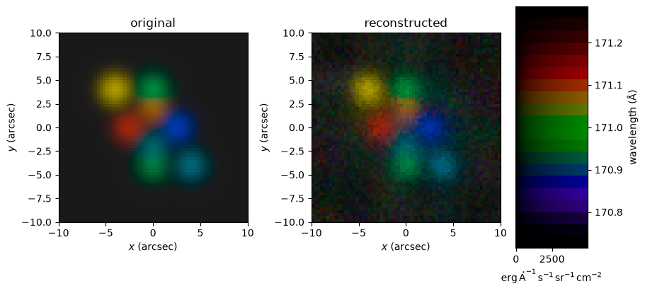
The hue of each pixel represents the Doppler shift of the spectral line, and the brightness represents its intensity.
Documentation
The full documentation, including the API reference, tutorials, and discussions of the theory behind the inversions, is hosted at ctis.readthedocs.io.
Citation
If you use ctis in your research, please cite it.
The citation metadata is kept in CITATION.cff,
which the "Cite this repository" button on GitHub can export as BibTeX or APA.
Every release of ctis is archived on Zenodo with its own DOI.
The concept DOI, 10.5281/zenodo.23086313,
always resolves to the latest version,
and the Zenodo page lists the DOI of every version.
Please include the version of ctis that you used,
which is given by importlib.metadata.version("ctis").
The BibTeX entry below uses the concept DOI.
To cite a specific version instead,
replace doi with the DOI of that version.
@software{ctis,
  author = {Smart, Roy T. and Parker, Jacob D. and Kankelborg, Charles C.},
  title = {ctis},
  version = {X.Y.Z},
  doi = {10.5281/zenodo.23086313},
  url = {https://github.com/sun-data/ctis},
}
Development
Install the package in editable mode along with its test dependencies, and run the test suite using pytest:
pip install -e .[test]
pytest
This project is formatted using black and linted using ruff, both of which are checked by continuous integration:
black .
ruff check .
To build the documentation locally:
pip install -e .[doc]
sphinx-build docs docs/_build/html
1 maintainer

Metadata
1 maintainer
Release files for ctis 0.5.1
For a detailed explanation of source distributions (sdists) and built distributions (wheels), please see the package formats documentation.
Source distribution (sdist)
| File | Size | Uploaded | |
|---|---|---|---|
| ctis-0.5.1.tar.gz | 78.1 kB | Details |
Built distribution (wheel)
| File | Interpreter | ABI | Platform | Reset |
|---|---|---|---|---|
| ctis-0.5.1-py3-none-any.whl | Python 3 | none | any | Details |
Total release size: 115.8 kB
Release files / ctis-0.5.1.tar.gz
| Download URL | ctis-0.5.1.tar.gz |
|---|---|
| Size | 78.1 kB |
| Tags | Source |
|
SHA-256 checksum How to use checksums |
891d4d99f66f4a6da57811a89d1a8334a07356073fd34b314b478c5632520afc
|
|
BLAKE2b-256 checksum How to use checksums |
de022a7758c3ff9e1d101e2e6145d54c9f13becaec0fa57f466e8ae1741577c8
|
| Upload date | |
|
Uploaded using Trusted Publishing? What is trusted publishing? |
Yes |
| Uploaded via |
twine/7.0.0 CPython/3.13.14
|
Provenance
Provenance describes where a file came from. On PyPI, provenance is shared via attestations, which provide a verifiable record of the build or publishing details. View details, limitations and caveats.


PyPI Publish Attestation
PyPI verified that this artifact, at this checksum, originated from the publisher listed below.
Signed by GitHub Actions, verified by PyPI on Oct 8, 2026.
Transparency logRelease files / ctis-0.5.1-py3-none-any.whl
| Download URL | ctis-0.5.1-py3-none-any.whl |
|---|---|
| Size | 37.7 kB |
| Tags | Python 3 |
|
SHA-256 checksum How to use checksums |
04316272b5be7879e9e0a8d618cf9065e6561bf08a4682e4b412ee653edfbb04
|
|
BLAKE2b-256 checksum How to use checksums |
28729c53b961f3bb212d8528e52ba36eb1fd9c7ed023df2e8a3f1b1db9830c2e
|
| Upload date | |
|
Uploaded using Trusted Publishing? What is trusted publishing? |
Yes |
| Uploaded via |
twine/7.0.0 CPython/3.13.14
|
Provenance
Provenance describes where a file came from. On PyPI, provenance is shared via attestations, which provide a verifiable record of the build or publishing details. View details, limitations and caveats.
PyPI Publish Attestation
PyPI verified that this artifact, at this checksum, originated from the publisher listed below.
Signed by GitHub Actions, verified by PyPI on Oct 8, 2026.
Transparency log













