
A Pure Python Clean-Room Implementation of the Fast Discrete Curvelet Transform

Project description
CurvePy: Fast Discrete Curvelet Transform (FDCT)




CurvePy is a pure Python "clean room" implementation of the Fast Discrete Curvelet Transform via Uniform Wrapping outlined in Emmanuel Candès 2005 paper Fast Discrete Curvelet Transforms
Unlike wavelets, which represent images using points, Curvelets represent images using oriented edges. This makes CurvePy (or the FDCT) a powerful tool for sparse representations of smooth curves, and highly effective at denoising while preserving sharp boundaries.
Results
Denoising
Grayscale images (2-D)
RGB images (3-D)
Curvepy uses a color denoising engine that operatues in the YUV color space (chosen to preserve structural details) while filtering chromatic noise.
Features
- Fast Discrete Curvelet Transform (FDCT): Implemented via the "wrapping" method outlined in Candès et al. 2005 for computational efficiency ($O(N^2 \log N)$).
- Color Support: wrapper specifically for RGB images using YUV separation. Processing Luma and Chroma channels independently.
- Thresholding Design:
- Soft Thresholding: For artifact-free restoration.
- Monte Carlo Calibration: Estimates noise levels per wedge and per scale.
- Module Design: Separates geometry computations, windowing and filtering logic into different modules.
Installation
Clone the repository and install the dependencies:
git clone [https://github.com/yourusername/curvepy.git](https://github.com/yourusername/curvepy.git)
cd curvepy
pip install -r requirements.txt
Usage
1. Basic Transformation (Grayscale image)
import matpolotlib.pyplot as plt
import skimage.data as data
from curvepy.curvepy import CurveletFrequencyGrid


# Initialize the Transformation engine (512x512 grid, 4 scales)
fdct = CurveletFrequencyGrid(N=512, scales=4)

# Load Image
image = data.camera()

# 1. Forward Transform
coefficients = fdct.forward_transform(image)

# 2. Inverse Transform
reconstructed_image = fdct.inverse_transform(coefficients)

# 3. Plot results
plt.figure(figsize=(12,4))
plt.suptitle("Original vs Reconstructed Image")

plt.subplot(1,2,1)
plt.imshow(image, plt.cmap.gray)
plt.title("Original")

plt.subplot(1,2,2)
plt.imshow(reconstructed_image, plt.cmap.gray)
plt.title("Restored Image")

plt.tight_layout()
plt.show()
2. Basic Transformation and Denoising (Grayscale image)
import matpolotlib.pyplot as plt
import skimage.data as data
from curvepy.curvepy import CurveletFrequencyGrid
from curvepy.denoise import CurveletDenoise


# Initialize the Transformation engine (512x512 grid, 4 scales)
fdct = CurveletFrequencyGrid(N=512, scales=4)
denoise_engine = CurveletDenoise(fdct)

# Load Image
image = data.camera()

# 1. Forward Transform
coefficients = fdct.forward_transform(image)

# 2. Denoise
restored_img = denoise_engine.denoise(noisy_img, sigma, multiplier)
psnr = denoise_engine.calculate_psnr_rgb(img, restored_img)

# 3. Plot results
plt.figure(figsize=(12,4))
plt.suptitle(f"Original vs restored img for soft thresholding, PSNR = {psnr:.2f} dB, multiplier = {multiplier}")

plt.subplot(1, 2, 1)
plt.imshow(img, cmap=plt.cm.gray)
plt.title("original img")

plt.subplot(1, 2, 2)
plt.imshow(restored_img, cmap=plt.cm.gray)
plt.title("restored img")

plt.tight_layout()
plt.show()
3. Denoising a Color Image
import matplotlib.pyplot as plt
import skimage.data as data
from curvepy.curvepy import CurveletFrequencyGrid
from curvepy.denoise import ColorCuerveletDenoise

# Setup
fdct = CurveletFrequencyGrid(N=512, scales=4)
denoise_engine = CuerveletDenoise(fdct)
image = denoise_engine.normalize_img(data.astronaut())

# Apply denoising
restored_image = denoise_engine.denoise(image, sigma=0.1, multiplier=1.5)
psnr = denoise_engine.calculate_psnr_rgb(image, restored_image) # Calculate peak SNR value between two images

# Plot results
plt.figure(figsize=(12,4))
plt.suptitle(f"Original vs Restored image via Soft Thresholding, PSNR = {psnr:.2f} dB, multiplier = {multiplier}")

plt.subplot(1, 2, 1)
plt.imshow(img)
plt.title("original img")

plt.subplot(1, 2, 2)
plt.imshow(restored_img)
plt.title("restored img")

plt.tight_layout()
plt.show()
4. Seismic Data Processing (SEG-Y & Compression)
CurvePy now supports direct SEG-Y ingestion and specialized seismic denoising. This pipeline demonstrates loading, aggressive denoising (targeting 95%+ sparsity), and quantization for massive compression savings.
import numpy as np
from curvepy.io import SeismicLoader
from curvepy.curvepy import CurveletFrequencyGrid
from curvepy.denoise import SeismicDenoise

# 1. Setup & Load
loader = SeismicLoader('path/to/data.sgy')
image = loader.load_2d_slice(inline=100)

grid = CurveletFrequencyGrid(nrows=image.shape[0], ncols=image.shape[1], scales=5)
denoiser = SeismicDenoise(grid)

# 2. Aggressive Denoising & Sparsity Check
# Returns clean image, sparsity %, and clean coefficients
clean_image, sparsity, clean_coeffs = denoiser.denoise(image, sigma=3.5)
print(f"Achieved Sparsity: {sparsity:.2f}%")

# 3. Quantization & Compression
# Save coefficients directly to HDF5 (often achieving 10x-20x compression ratios)
loader.save_quantized_coefficients(clean_coeffs, 'path/to/data.h5', threshold=0)
5. Scientific Signal Analysis (Synthetic ANT)
This example generates a dispersive surface wave, adds noise, and recovers the signal while preserving the Frequency-Wavenumber (F-K) spectrum.
import numpy as np
import matplotlib.pyplot as plt
from curvepy.curvepy import CurveletFrequencyGrid
from curvepy.denoise import SeismicDenoise

# Generate Synthetic Dispersive Wave
rows, cols = 256, 256
t = np.linspace(-2, 2, rows)
x = np.linspace(0, 5, cols)
T, X = np.meshgrid(t, x, indexing='ij')

# Signal: Clean dispersive arc + heavy Gaussian noise
clean_signal = np.sin(2 * np.pi * 5 * (T - 0.1 * X**2)) * np.exp(-10 * (T - 0.1 * X**2)**2)
noisy_data = clean_signal + 0.8 * np.random.randn(rows, cols)

# Denoise
grid = CurveletFrequencyGrid(rows, cols, scales=5)
denoiser = SeismicDenoise(grid)
denoised, sparsity, _ = denoiser.denoise(noisy_data, sigma=2.5)
Project Structure
curvepy/
├── curvepy.py # Core Engine: FDCT & IFDCT implementation
├── windows.py # Math: Meyer Window functions (Phi, Psi, V)
├── filters.py # Tools: Thresholding logic & Monte Carlo calibration
├── denoise.py # App: Seismic & Color Denoising pipelines
└── io.py # Tools: SEG-Y Loading & HDF5 Compression
Theory + How it Works:
Standard 2D Wavelets are isotropic, ie. they treat all directions equally. This doens't work well for images where the curves/outlines of the shapes are what are important to be preserved. This creates a blocky or ringing effect when trying to represent a smooth curve.
Curvelets are anisotropic "needles" that exist at different scales and angles
- Scales: Captures details of different sizes.
- Angles: Capture the direction of the geometry.
This allows CurvePy to represent a curved edge with very few coefficients relative to the aformentioneed 2D wavelets, making it ideal for compression and restoration tasks while preserving the geometry is important :)
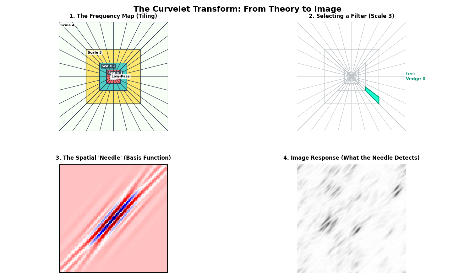
To understand why this matters, we visualized the inner workings of the transform below:
Image
The 4-Step Pipeline (Explained)
-
The Map (Top-Left): The Frequency Plane is tiled into "Wedges." Each wedge represents a specific combination of Scale (how thick the feature is) and Angle (which way it points).
- Center (Grey): Low-frequency background (blurry shapes).
- Outer Rings (Colors): High-frequency details (sharp edges).
-
The Filter (Top-Right): To detect specific features, we activate just one single wedge. In this example, we selected Scale 3, Wedge 0. This filter is specialized to find "Medium-Fine details that are Horizontal."
-
The Needle (Bottom-Left): This is what that single filter looks like in the real world (Spatial Domain). It isn't a point—it's a Needle.
-
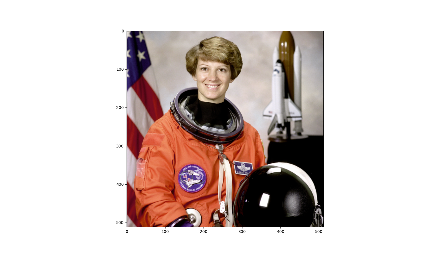
The Response (Bottom-Right): When we drag this Needle across a real photo (The Astronaut), it lights up (turns black) only where it finds matching geometry.
- Notice the top of the helmet and the flag stripes are clearly visible because they are horizontal.
- The vertical rocket boosters in the background are invisible. The horizontal needle doesn't notice the vertical lines.
Visual Proofs & Benchmarks
1. Physics Preservation (F-K Spectrum)
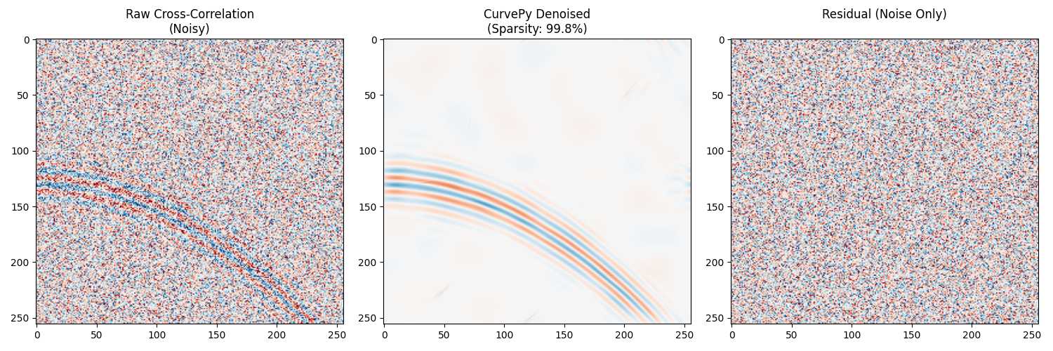
One of CurvePy's primary goals is to denoise without destroying the underlying physics of the signal.
- Left: The raw cross-correlation with heavy noise.
- Center: The denoised output.
- Right: The Residual (Noise) containing no coherent structural energy.
2. Spectral Integrity
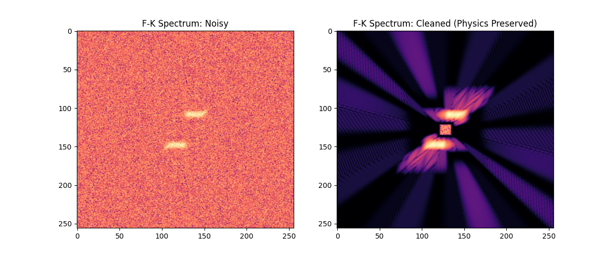
Comparing the F-K (Frequency-Wavenumber) spectrum before and after denoising confirms that the relevant frequency content is preserved while incoherent noise is rejected.
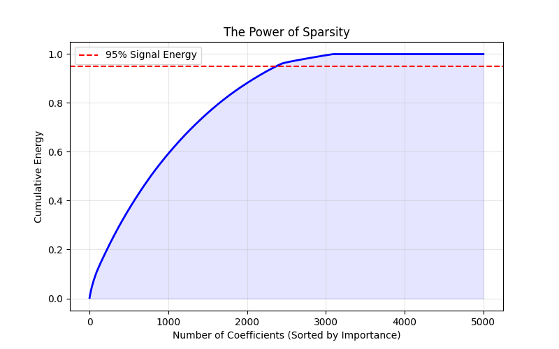
3. The Power of Sparsity
Curvelets represent curve-like geometry extremely efficiently. As shown below, 95% of the signal energy is often contained in a tiny fraction of the coefficients. This is the mechanism that allows for high-ratio compression.
Licence
MIT Licence. Free to use for academic and personal projects.


Download files
Download the file for your platform. If you're not sure which to choose, learn more about installing packages.
Source Distribution
Built Distribution
Filter files by name, interpreter, ABI, and platform.
If you're not sure about the file name format, learn more about wheel file names.
Copy a direct link to the current filters
File details
Details for the file curvepy_fdct-1.1.1.tar.gz.
File metadata
- Download URL: curvepy_fdct-1.1.1.tar.gz
- Upload date:
- Size: 197.8 kB
- Tags: Source
- Uploaded using Trusted Publishing? No
- Uploaded via: poetry/2.3.2 CPython/3.14.3 Darwin/24.4.0
File hashes
| Algorithm | Hash digest | |
|---|---|---|
| SHA256 |
5371e0f7ac7cec16e092f86240eefcd3a081c37a2229d9a7718dcd13d13f8f67
|
|
| MD5 |
c9f3d7c2f237ce945f898a6b2f056ff4
|
|
| BLAKE2b-256 |
0cd2d48c05e8455c0a1e543b3178a7e2a59b07a45b6d4429cec3766c7ef20bce
|
File details
Details for the file curvepy_fdct-1.1.1-cp314-cp314-macosx_15_0_x86_64.whl.
File metadata
- Download URL: curvepy_fdct-1.1.1-cp314-cp314-macosx_15_0_x86_64.whl
- Upload date:
- Size: 284.3 kB
- Tags: CPython 3.14, macOS 15.0+ x86-64
- Uploaded using Trusted Publishing? No
- Uploaded via: poetry/2.3.2 CPython/3.14.3 Darwin/24.4.0
File hashes
| Algorithm | Hash digest | |
|---|---|---|
| SHA256 |
1aa8f9b38849d392d1828653cdb940223112a69d034200a8b537327c81395e7a
|
|
| MD5 |
38cfdd8f8254d0861c702beee894ab1c
|
|
| BLAKE2b-256 |
b6f541aea89f6e252b8120f8818c0894f41ea9c8ae2b9513d4c82bb3a1158a60
|






