Datawaza is a collection of tools for data exploration, visualization, data cleaning, pipeline creation, model iteration, and evaluation.

Project description


Datawaza streamlines common Data Science tasks. It's a collection of tools for data exploration, visualization, data cleaning, pipeline creation, hyper-parameter searching, model iteration, and evaluation. It builds upon core libraries like Pandas, Matplotlib, Seaborn, and Scikit-Learn.
Installation
The latest release can be found on PyPI. Install Datawaza with pip:
pip install datawaza
See the Change Log for a history of changes.
Dependencies
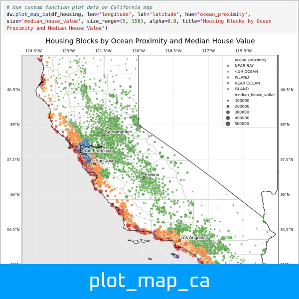
Datawaza supports Python 3.9 - 3.12. Because Cartopy does not support Python 3.8, and that's a dependency for plot_map_ca, 3.8 is not supported.
Installation requires NumPy, Pandas, Matplotlib, Seaborn, Plotly, Scikit-Learn, SciPy, Cartopy, GeoPandas, StatsModels, TensorFlow, Keras, SciKeras (if utilizing KerasClassifier as a model), PyTorch, and a few other supporting packages. See the Requirements.txt.
Documentation
Online documentation is available at Datawaza.com.
The User Guide is a Jupyter notebook that walks through how to use the Datawaza functions. It's probably the best place to start. There is also an API reference for the major modules: Clean, Explore, Model, and Tools.
Development
The Datawaza repo is on GitHub.
Please submit bugs that you encounter to the Issue Tracker. Contributions and ideas for enhancements are welcome!
What is Waza?
Waza (技) means "technique" in Japanese. In martial arts like Aikido, it is paired with words like "suwari-waza" (sitting techniques) or "kaeshi-waza" (reversal techniques). So we've paired it with "data" to represent Data Science techniques: データ技 "data-waza".
Origin Story
Most of these functions were created while I was pursuing a Professional Certificate in Machine Learning & Artificial Intelligence from U.C. Berkeley. With each assignment, I tried to simplify repetitive tasks and streamline my workflow. They served me well at the time, so perhaps they will be of value to others.
Quick Start
The User Guide will show you how to use Datawaza's functions in depth. Assuming you already have data loaded, here are some examples of what it can do:
>>> import datawaza as dw
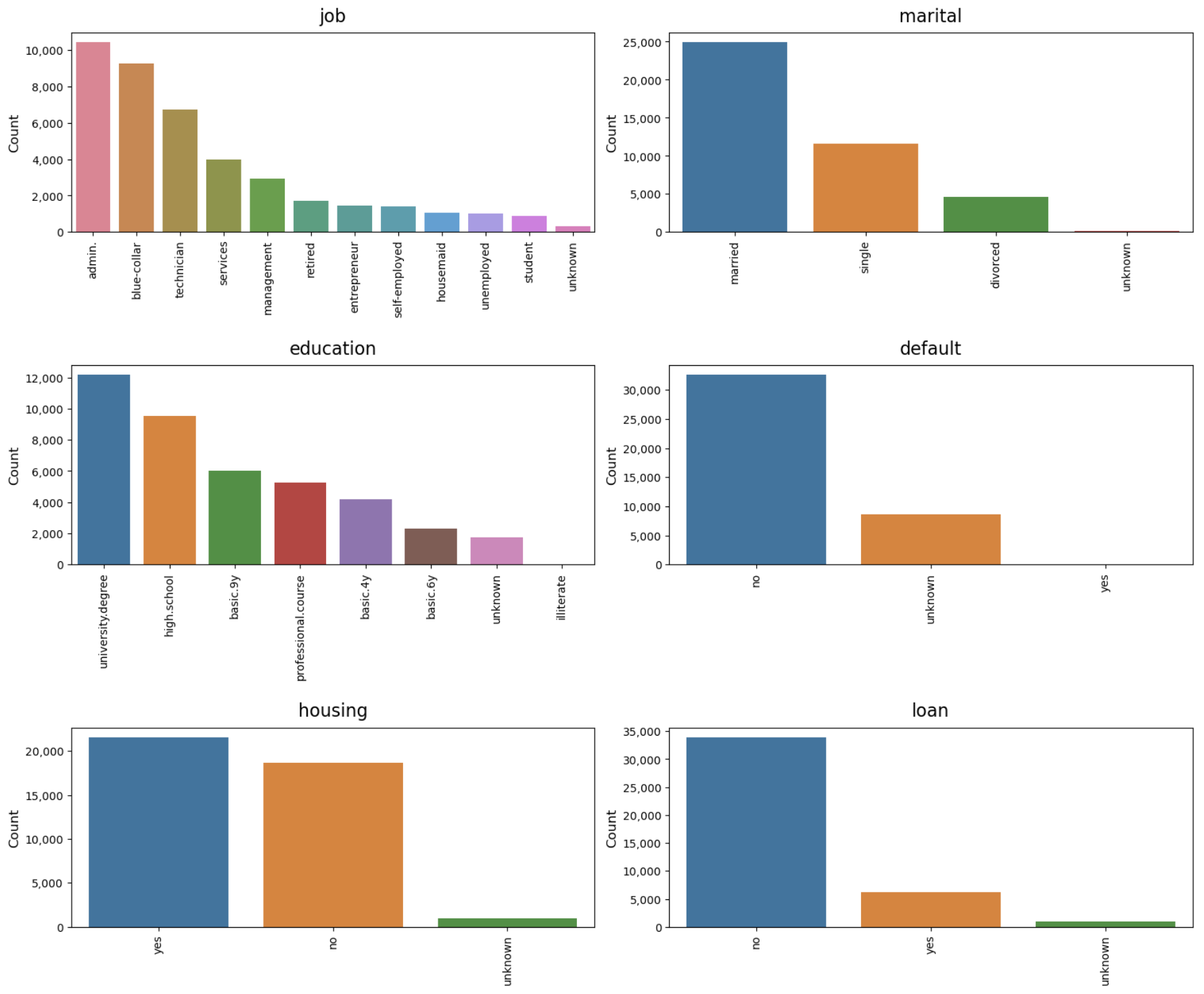
Show the unique values of each variable below the threshold of n = 12:
>>> dw.get_unique(df, 12, count=True, percent=True)

CATEGORICAL: Variables with unique values equal to or below: 12

job has 12 unique values:

    admin.              10422   25.3%
    blue-collar         9254    22.47%
    technician          6743    16.37%
    services            3969    9.64%
    management          2924    7.1%
    retired             1720    4.18%
    entrepreneur        1456    3.54%
    self-employed       1421    3.45%
    housemaid           1060    2.57%
    unemployed          1014    2.46%
    student             875     2.12%
    unknown             330     0.8%

marital has 4 unique values:

    married        24928   60.52%
    single         11568   28.09%
    divorced       4612    11.2%
    unknown        80      0.19%
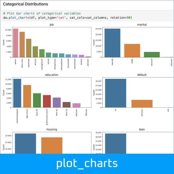
Plot bar charts of categorical variables:
>>> dw.plot_charts(df, plot_type='cat', cat_cols=cat_columns, rotation=90)
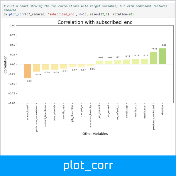
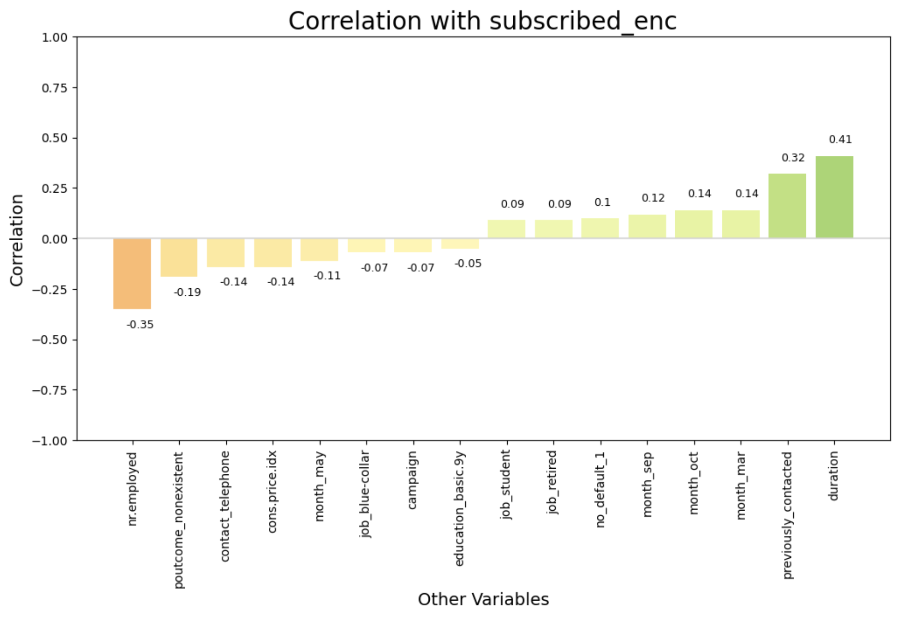
Get the top positive and negative correlations with the target variable, and save to lists:
>>> pos_features, neg_features = dw.get_corr(df_enc, n=10, var='subscribed_enc', return_arrays=True)

Top 10 positive correlations:
              Variable 1      Variable 2  Correlation
0               duration  subscribed_enc         0.41
1       poutcome_success  subscribed_enc         0.32
2   previously_contacted  subscribed_enc         0.32
3                  pdays  subscribed_enc         0.27
4               previous  subscribed_enc         0.23
5              month_mar  subscribed_enc         0.14
6              month_oct  subscribed_enc         0.14
7              month_sep  subscribed_enc         0.12
8           no_default_1  subscribed_enc         0.10
9            job_student  subscribed_enc         0.09

Top 10 negative correlations:
              Variable 1      Variable 2  Correlation
0            nr.employed  subscribed_enc        -0.35
1              euribor3m  subscribed_enc        -0.31
2           emp.var.rate  subscribed_enc        -0.30
3   poutcome_nonexistent  subscribed_enc        -0.19
4      contact_telephone  subscribed_enc        -0.14
5         cons.price.idx  subscribed_enc        -0.14
6              month_may  subscribed_enc        -0.11
7               campaign  subscribed_enc        -0.07
8        job_blue-collar  subscribed_enc        -0.07
9     education_basic.9y  subscribed_enc        -0.05
Plot a chart showing the top correlations with the target variable:
>>> dw.plot_corr(df_enc, 'subscribed_enc', n=16, size=(12,6), rotation=90)
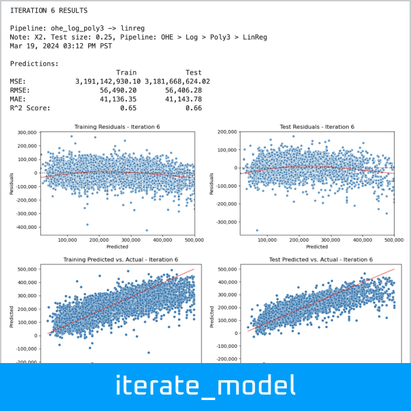
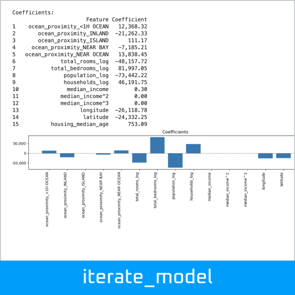
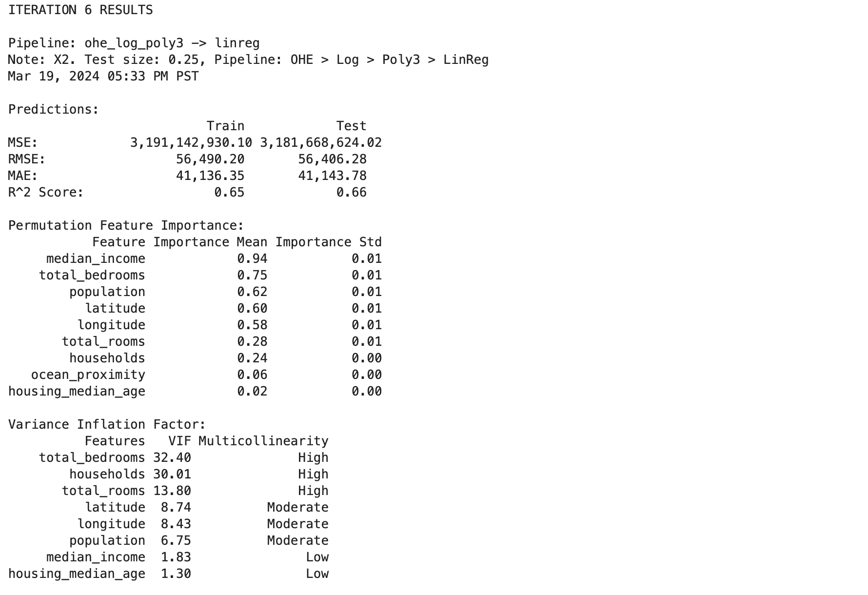
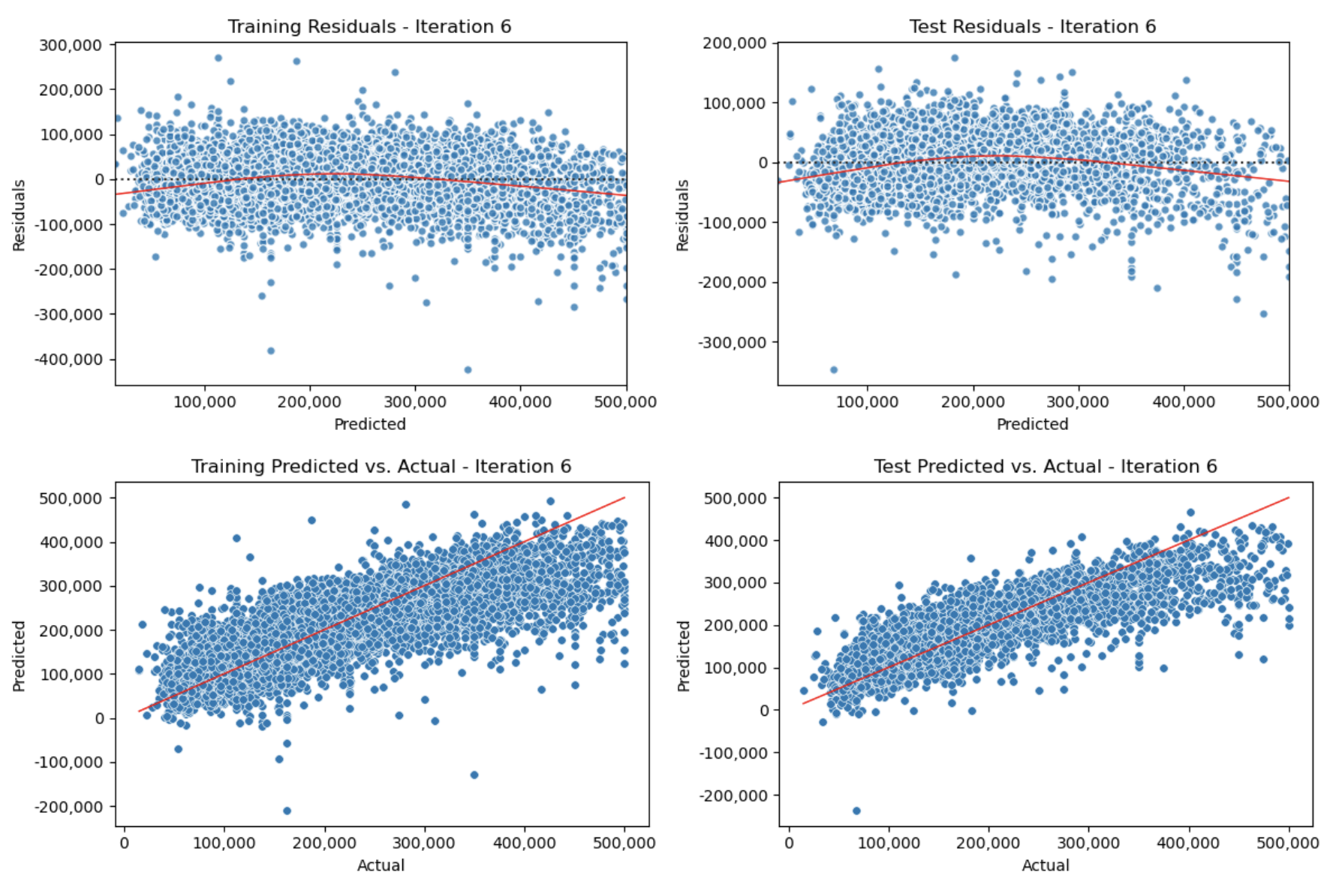
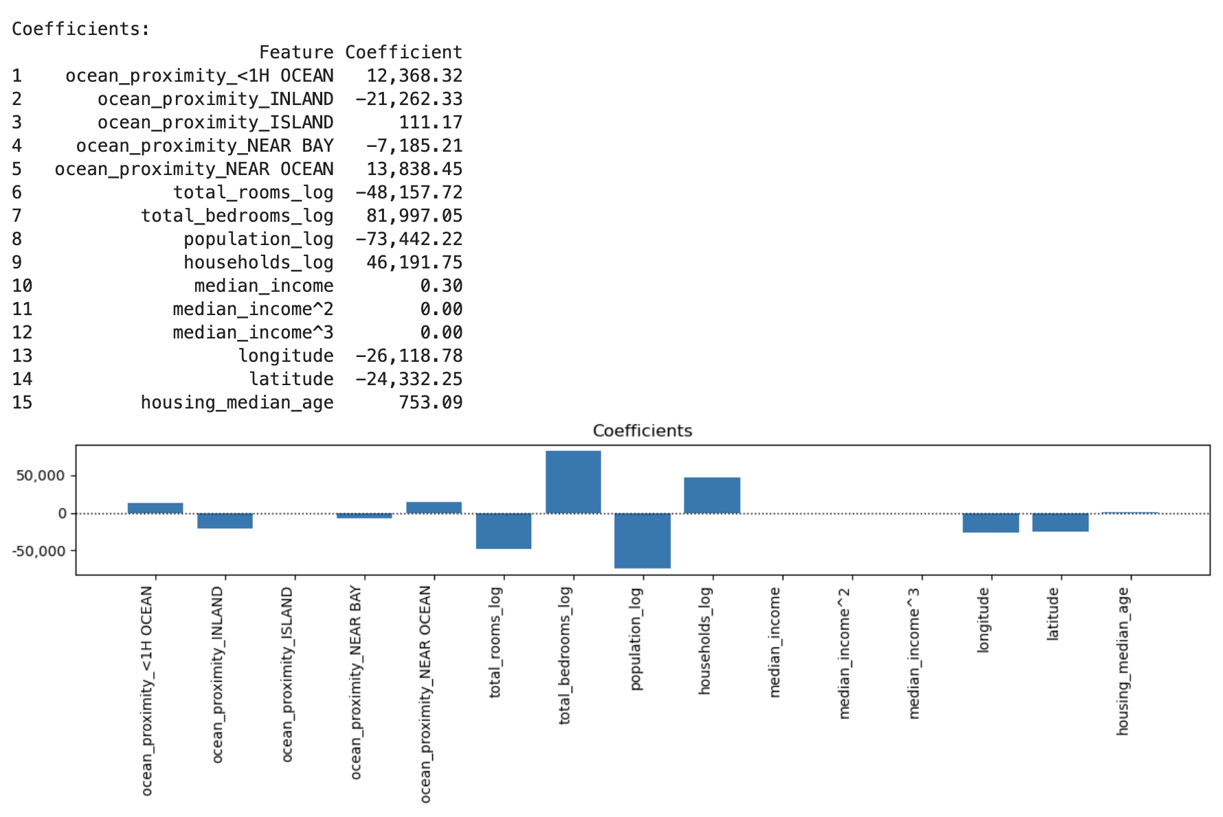
Run a regression model iteration, which dynamically assembles a pipeline and evaluates the model, including charts of residuals, predicted vs. actual, and coefficients:
>>> results_df, iteration_6 = dw.iterate_model(X2_train, X2_test, y2_train, y2_test,
...     transformers=['ohe', 'log', 'poly3'], model='linreg',
...     iteration='6', note='X2. Test size: 0.25, Pipeline: OHE > Log > Poly3 > LinReg',
...     plot=True, lowess=True, coef=True, perm=True, vif=True, decimal=2,
...     save=True, save_df=results_df, config=my_config)
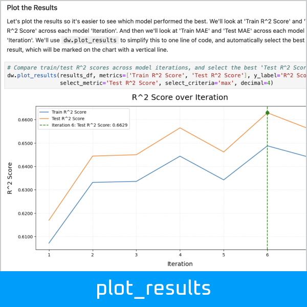
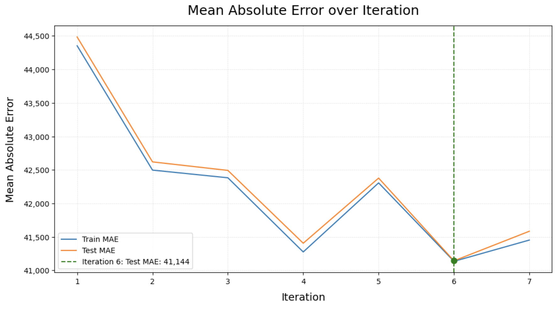
Compare train/test scores across model iterations, and select the best result:
>>> dw.plot_results(results_df, metrics=['Train MAE', 'Test MAE'], y_label='Mean Absolute Error',
...     select_metric='Test MAE', select_criteria='min', decimal=0)
Define a configuration file to compare multiple binary classification models:
>>> # Set some variables referenced in the config
>>> random_state = 42
>>> class_weight = None
>>> max_iter = 10000
>>>
>>> # Set column lists referenced in the config
>>> num_columns = list(X.columns)
>>> cat_columns = []
>>>
>>> # Create a custom configuration file with 3 models and grid search params
>>> my_config = {
...     'models' : {
...         'logreg': LogisticRegression(max_iter=max_iter,
...                   random_state=random_state, class_weight=class_weight),
...         'knn_class': KNeighborsClassifier(),
...         'tree_class': DecisionTreeClassifier(random_state=random_state,
...                       class_weight=class_weight)
...     },
...     'imputers': {
...         'simple_imputer': SimpleImputer()
...     },
...     'transformers': {
...         'ohe': (OneHotEncoder(drop='if_binary', handle_unknown='ignore'),
...                     cat_columns)
...     },
...     'scalers': {
...         'stand': StandardScaler()
...     },
...     'selectors': {
...         'sfs_logreg': SequentialFeatureSelector(LogisticRegression(
...                       max_iter=max_iter, random_state=random_state,
...                       class_weight=class_weight))
...     },
...     'params' : {
...         'logreg': {
...             'logreg__C': [0.0001, 0.001, 0.01, 0.1, 1, 10, 100],
...             'logreg__solver': ['newton-cg', 'lbfgs', 'saga']
...         },
...         'knn_class': {
...             'knn_class__n_neighbors': [3, 5, 10, 15, 20, 25],
...             'knn_class__weights': ['uniform', 'distance'],
...             'knn_class__metric': ['euclidean', 'manhattan']
...         },
...         'tree_class': {
...             'tree_class__max_depth': [3, 5, 7],
...             'tree_class__min_samples_split': [5, 10, 15],
...             'tree_class__criterion': ['gini', 'entropy'],
...             'tree_class__min_samples_leaf': [2, 4, 6]
...         },
...     },
...     'cv': {
...         'kfold_5': KFold(n_splits=5, shuffle=True, random_state=42)
...     },
...     'no_scale': ['tree_class'],
...     'no_poly': ['knn_class', 'tree_class']
... }
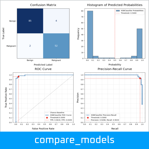
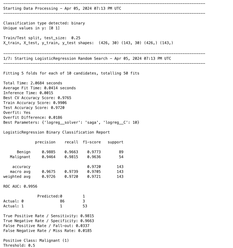
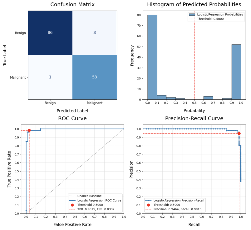
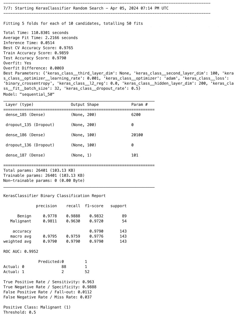
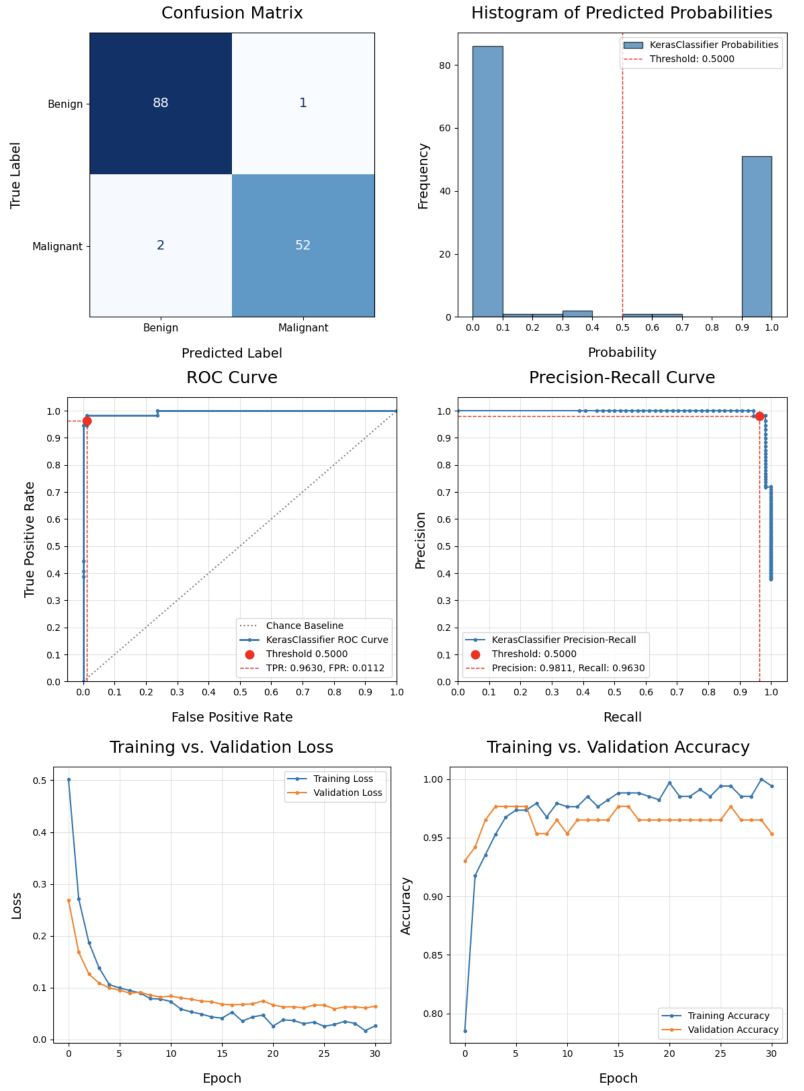
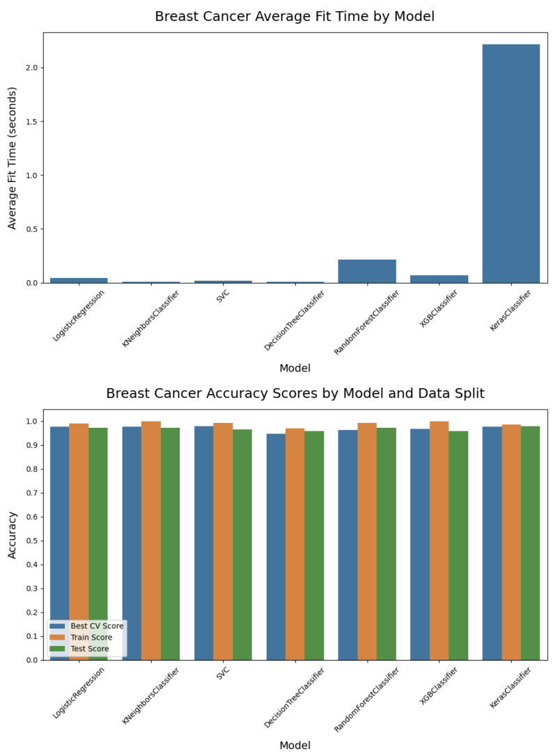
Run a binary classification on 7 models, dynamically assembling the pipeline and performing a grid search of the hyper-parameters, all based on the configuration file defined above:
>>> results_df = compare_models(
...
...     # Data split and sampling
...     x=X, y=y, test_size=0.25, stratify=None, under_sample=None,
...     over_sample=None, svm_knn_resample=None,
...
...     # Models and pipeline steps
...     imputer=None, transformers=None, scaler='stand', selector=None,
...     models=['logreg', 'knn_class', 'svm_proba', 'tree_class',
...     'forest_class', 'xgb_class', 'keras_class'], svm_proba=True,
...
...     # Grid search
...     search_type='random', scorer='accuracy', grid_cv='kfold_5', verbose=1,
...
...     # Model evaluation and charts
...     model_eval=True, plot_perf=True, plot_curve=True, fig_size=(12,6),
...     legend_loc='lower left', rotation=45, threshold=0.5,
...     class_map=class_map, pos_label=1, title='Breast Cancer',
...
...     # Config, preferences and notes
...     config=my_config, class_weight=None, random_state=42, decimal=4,
...     n_jobs=None, notes='Test Size=0.25, Threshold=0.50'
... )  #doctest: +NORMALIZE_WHITESPACE
This was just a sample of some Datawaza tools. Download userguide.ipynb and explore the full breadth of the library in your Jupyter environment.
Release history Release notifications | RSS feed


Download files
Download the file for your platform. If you're not sure which to choose, learn more about installing packages.
Source Distribution
Built Distribution
Filter files by name, interpreter, ABI, and platform.
If you're not sure about the file name format, learn more about wheel file names.
Copy a direct link to the current filters
File details
Details for the file datawaza-0.1.3.tar.gz.
File metadata
- Download URL: datawaza-0.1.3.tar.gz
- Upload date:
- Size: 4.4 MB
- Tags: Source
- Uploaded using Trusted Publishing? No
- Uploaded via: twine/5.0.0 CPython/3.10.13
File hashes
| Algorithm | Hash digest | |
|---|---|---|
| SHA256 |
3429eaa92a13f39ae10f3e67adba3ba39b0cbd4677d740c1f06751dc3d790440
|
|
| MD5 |
cc82437aaddfe1856d0ae1753b90ddc4
|
|
| BLAKE2b-256 |
80cb40281e5e6f0d8db0dbc5421ab39bbd33e1c711e3a8cdba4ccbe86a6724cf
|
File details
Details for the file datawaza-0.1.3-py3-none-any.whl.
File metadata
- Download URL: datawaza-0.1.3-py3-none-any.whl
- Upload date:
- Size: 4.4 MB
- Tags: Python 3
- Uploaded using Trusted Publishing? No
- Uploaded via: twine/5.0.0 CPython/3.10.13
File hashes
| Algorithm | Hash digest | |
|---|---|---|
| SHA256 |
e0c4afef557d621563736186f5db4720b70d8fc796a771f4f2bc74352bf50f62
|
|
| MD5 |
81b48d23287ac7912604cc6a6836008f
|
|
| BLAKE2b-256 |
e710d0bdd5b51f78ae18137b920ba93b2949f7b8f128eeadb797a2d1d03940d3
|


