
DBCV-revisited
⚡ A Memory-Efficient, High-Performance Implementation of Density-Based Cluster Validation
Provides 20X+ speedup consistently compared to other available options, while using less than one-quarter of the peak memory on moderate to large datasets.
Also matches the score of the MATLAB reference implementation up to floating-point noise beyond 10 decimal places.
Table of Contents
Why DBCV?
Think of ANOVA:
$$ \boldsymbol{F} = \frac{ MS_{\text{between}} }{ MS_{\text{within}} } $$
The underlying idea is simple: well-defined groups should exhibit low variation internally and clear separation from one another.
However, when groups have arbitrary shapes, a centroid may be a poor representation of the observations they contain. This is particularly relevant for density-based methods such as HDBSCAN, which can identify non-convex, elongated, and otherwise irregular structures. As a result, validity measures based on distances to cluster centroids may fail to capture their true geometry.
This is where Density-Based Cluster Validation (DBCV) comes in.
DBCV follows the same fundamental principle of balancing internal compactness against external separation, but does so without assuming a particular geometric shape. It constructs a Minimum Spanning Tree (MST) for each group to characterize its internal density structure via the maximum-weight edge, and uses cross-MST distances to quantify the separation between groups.
For a clustering of dataset $\mathcal{X}$ into clusters $C_1, \dots, C_l$:
$$ \mathbf{DBCV}(\mathcal{X}) = \sum_{i=1}^{l} \frac{|C_i|}{|\mathcal{X}|} , \mathbf{V_C}(C_i) $$
where the validity of a single cluster $C_i$ balances its internal sparseness against its separation from the nearest other cluster:
$$ \boxed{ \boldsymbol{ V_C(C_i) = \frac{ \min\limits_{j \neq i} \text{DSPC}(C_i, C_j) - \text{DSC}(C_i) }{ \max\left( \min\limits_{j \neq i} \text{DSPC}(C_i, C_j), \text{DSC}(C_i) \right) } } } $$
$\text{DSC}(C_i)$ (Density Sparseness of a Cluster) and $\text{DSPC}(C_i, C_j)$ (Density Separation of a Pair of Clusters) are exactly the two MST-derived quantities named above — how we compute each is covered in our own contributions below. $|\mathcal{X}|$ includes noise points (they contribute $0$ to the sum, via no $C_i$ of their own), so a clustering that leaves more points unclassified as noise cannot inflate its score by only counting the points it did assign.
DBCV was originally proposed by Moulavi et al. (2014), as an improvement over the then widely used multi-representative-based CDbw index (Halkidi & Vazirgiannis, 2008). Subsequent comparative studies have shown that DBCV can outperform competing density-based validity indices and exhibit robust performance across a wide range of clustering scenarios, particularly for non-globular, concave, and density-based structures [Chicco et al., 2025; Simpson et al., 2026].
This makes DBCV particularly well suited to evaluating methods such as HDBSCAN, where density, rather than geometric shape, is central to how groups are identified.
Available Options
The time and space complexity of DBCV scales quadratically with the number of observations, which limits its adoption for large datasets.
The available CRAN implementation, dbscan, explicitly acknowledges this limitation in its documentation:
Performance note: This implementation calculates a distance matrix and thus can only be used for small or sampled datasets.
In Python, three notable implementations are:
HDBSCAN—validity_indexBundled with the widely used HDBSCAN package, this implementation uses an efficient Cython routine for MST construction. However, it explicitly materializes dense pairwise mutual-reachability matrices for density sparseness (DSC) and dense cross-cluster distance/MRD matrices for density separation (DSPC).FelSiq/DBCVThis vanilla implementation is designed to be "fully compatible with the original MATLAB implementation" and is commonly used in academic comparisons and benchmarks.k-DBCVThis implementation introduces a KD-tree-based spatial partitioning strategy in place of brute-force nearest-neighbor search. During our review, however, we identified an implementation inconsistency, which is documented in Issue #3 and was brought to the author's attention.
OUR CONTRIBUTION
Our Contribution: DSC (Density Sparseness of a Cluster)
The typical workflow for DSC is, for each cluster $i$:
Step 1: Computes the Euclidean distance matrix. | Incremental memory: $O(n_i^2)$
Step 2: Computes the all-points-core-distance array. | Incremental memory: $O(n_i)$
Step 3: Computes the mutual-reachability distance matrix. | Incremental memory: $O(n_i^2)$
Step 4: Computes the minimum spanning tree. | Incremental memory: $O(n_i-1)$
We have made the following optimizations:
Step 1:
Computes only the upper-triangular block of the Euclidean distance matrix and stores it in a condensed array format (see SciPy's pdist). The distance matrix is symmetric by definition, with zero-valued diagonals, so there is no reason to ever materialize the full matrix. |
Incremental memory: $O(n_i(n_i-1)/2)$
Step 2:
Computes the all-points-core-distance array as is. |
Incremental memory: $O(n_i)$
Step 3:
The Euclidean and mutual-reachability distance matrices have exactly the same shape, and the argument about diagonal symmetry still holds. We update the allocation from Step-1 in place. |
Incremental memory: $0$
Step 4:
Computes the minimum spanning tree. The available HDBSCAN implementations of Prim's algorithm only accept a full $n_i \times n_i$ distance matrix.
So, we customized the algorithm from scratch to work directly with the condensed array from Step-3, without ever materializing it in full squareform. |
Incremental memory: $O(n_i-1)$
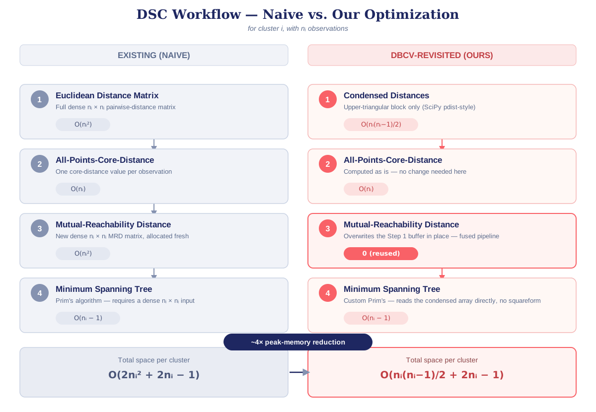
So, the total space complexity per cluster is reduced from $O(2n_i^2+2n_i-1)$ to $O\left(\frac{n_i(n_i-1)}{2}+2n_i-1\right)$. Although both are quadratic, this gives an approximately 4X peak-memory reduction in the constant factor for large $n_i$, theoretically guaranteed even before applying any other optimization.
Our Contribution: DSPC (Density Separation of a Pair of Clusters)
For DSPC, we adopt a KD-tree approach to avoid materializing cross-cluster matrices in a loop.
The tree is built from the combined data of core points from all clusters, and we need to find the nearest neighbor of a point outside its own cluster.
So, the typical workflow demonstrated in k-DBCV for cluster $i$ is:
Step 1: Find #cluster_core_size + 1 neighbors for each point to ensure at least one outside-cluster neighbor.
Step 2: Discard the same-cluster neighbors and retain only the closest outside-cluster neighbor using index filtering; we already know which observation ID belongs to which cluster.
Here, we patch the brute-force loop on the leaf nodes of the query routine to perform the index filtering before distance calculation. The internal-node tree traversal remains the same.
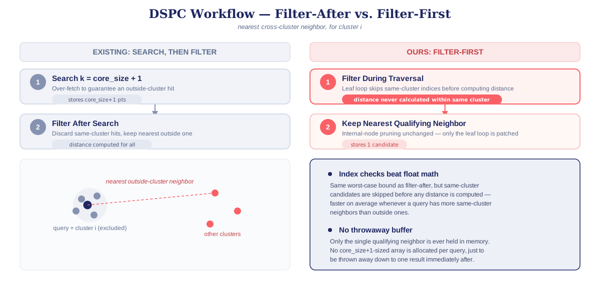
This modification gives us the following benefits:
- Index comparison is always cheaper than floating-point distance computation.
When we know in advance that a same-cluster observation is not required downstream, we can short-circuit the iteration without ever performing the distance arithmetic.
The worst-case upper bound for
(Step-1, Step-2)combined remains the same, because we are performing the same task, just in a different order. However, in most cases, where a query point is surrounded by more same-cluster observations than outside-cluster observations, this reduces the average runtime. - We no longer need to store
#cluster_core_size + 1neighbors per query in an intermediate array, only to discard all but one.
How to Use
pip install dbcv-revisit
Or,
git clone https://github.com/idnantimar/DBCV-revisited.git
cd DBCV-revisited
pip install .
Overall score only:
from sklearn.datasets import make_blobs
from DBCV import DBCV_score

X, y = make_blobs(n_samples=500, centers=4, random_state=0)
score = DBCV_score(X, y)
With per_cluster_scores=True, you additionally get each cluster's own contribution back as an array, alongside the overall score:
score, cluster_scores = DBCV_score(X, y, per_cluster_scores=True)
There is a n_jobs parameter to enable joblib.Parallel(...)-based multi-threading; however, the default single-threaded execution is generally sufficient, and you may barely need n_jobs in practice.
Beyond the top-level DBCV_score, we've also built and exposed two standalone utilities under DBCV.utils, usable independently of DBCV itself:
- MST (
mst_linkage_core_condensed) — Prim's algorithm operating directly on a condensed (upper-triangular) distance array, with nosquareformstep ever required. - KDTree (
cKDTree) — ascipy.spatial.cKDTreefork with traversal-level, index-based neighbor filtering, so cross-cluster nearest-neighbor queries never pay for a same-cluster distance calculation.
from DBCV.utils import mst_linkage_core_condensed, cKDTree
NOTE: There is no free lunch. By adding an extra layer of index manipulation in the $O(n_i^2)$ hot loop of Prim's algorithm, our customized MST routine should run slower than a generic MST builder when considered in isolation. However, we have optimized the complete DBCV workflow tightly enough to absorb those extra seconds and achieve a net positive runtime improvement.
Time & Memory
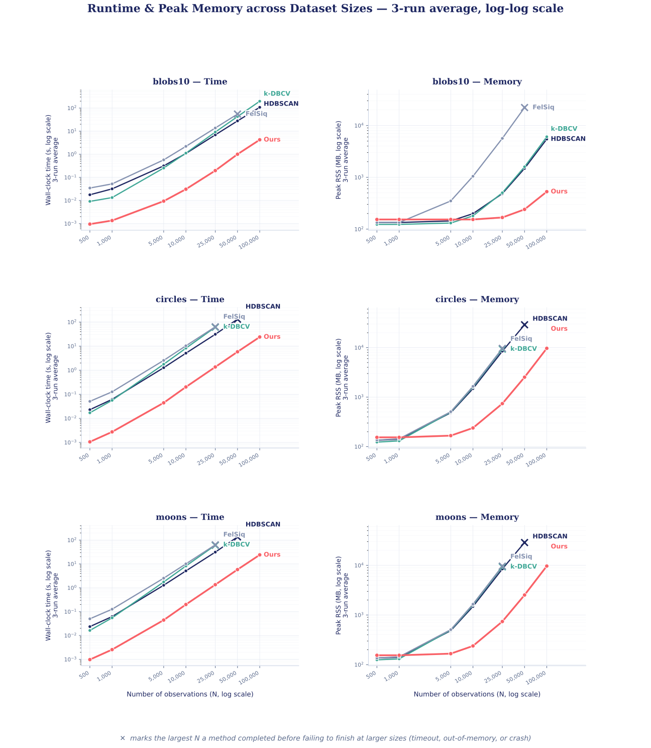
Wall-clock time and peak RSS, scaling from 500 to 100,000 observations:
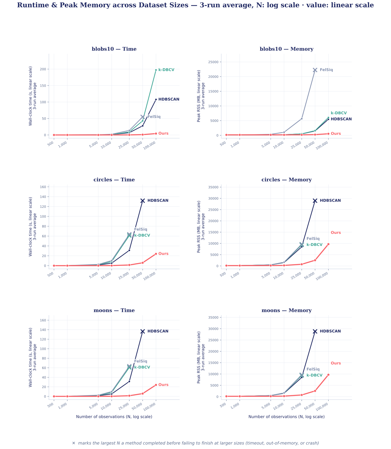
Keeping N on a log scale (so the smaller sizes stay readable) but switching the value axis to linear makes the gap even more visually stark.
Score
Agreement with felsiq's reference implementation:
Score for each dataset, method, and run, across all sizes. NA marks a run that did not finish at that size (timeout, out-of-memory, or crash) — same convention as the ✕ markers in Time & Memory.
blobs10
| method | run | 500 | 1,000 | 5,000 | 10,000 | 25,000 | 50,000 | 100,000 |
|---|---|---|---|---|---|---|---|---|
| Ours | 1 | 0.471676 | 0.159922 | 0.032993 | -0.155677 | -0.350667 | -0.320743 | -0.388716 |
| 2 | 0.393145 | 0.369820 | -0.048403 | -0.140218 | -0.263146 | -0.396820 | -0.388716 | |
| 3 | 0.556961 | 0.094470 | 0.134878 | 0.013771 | -0.229369 | -0.319273 | -0.388716 | |
| HDBSCAN | 1 | 0.342005 | 0.077528 | -0.098594 | -0.414285 | -0.453398 | -0.489233 | -0.641142 |
| 2 | 0.255302 | 0.230741 | -0.269673 | -0.293055 | -0.367287 | -0.620205 | -0.641142 | |
| 3 | 0.427322 | 0.012976 | -0.134381 | -0.147638 | -0.487128 | -0.431217 | -0.641142 | |
| FelSiq | 1 | 0.471676 | 0.159922 | 0.032993 | -0.155677 | -0.350667 | -0.320743 | NA |
| 2 | 0.393145 | 0.369820 | -0.048403 | -0.140218 | -0.263146 | -0.396820 | NA | |
| 3 | 0.556961 | 0.094470 | 0.134878 | 0.013771 | -0.229369 | -0.319273 | NA |
circles
| method | run | 500 | 1,000 | 5,000 | 10,000 | 25,000 | 50,000 | 100,000 |
|---|---|---|---|---|---|---|---|---|
| Ours | 1 | 0.852832 | 0.929685 | 0.966851 | 0.968470 | 0.986505 | 0.989319 | 0.990307 |
| 2 | 0.838167 | 0.928815 | 0.980886 | 0.938114 | 0.986037 | 0.989340 | 0.990307 | |
| 3 | 0.879361 | 0.938497 | 0.982724 | 0.983148 | 0.990684 | 0.984710 | 0.990307 | |
| HDBSCAN | 1 | 0.821221 | 0.902565 | 0.916952 | 0.944469 | 0.949026 | 0.928348 | NA |
| 2 | 0.803025 | 0.888394 | 0.913532 | 0.914954 | 0.945142 | 0.963527 | NA | |
| 3 | 0.869090 | 0.869601 | 0.905527 | 0.908973 | 0.934511 | 0.938836 | NA | |
| FelSiq | 1 | 0.852832 | 0.929685 | 0.966851 | 0.968470 | 0.986505 | NA | NA |
| 2 | 0.838167 | 0.928815 | 0.980886 | 0.938114 | 0.986037 | NA | NA | |
| 3 | 0.879361 | 0.938497 | 0.982724 | 0.983148 | 0.990684 | NA | NA |
moons
| method | run | 500 | 1,000 | 5,000 | 10,000 | 25,000 | 50,000 | 100,000 |
|---|---|---|---|---|---|---|---|---|
| Ours | 1 | 0.927630 | 0.962210 | 0.977990 | 0.946061 | 0.951122 | 0.968099 | 0.943718 |
| 2 | 0.812001 | 0.950442 | 0.972039 | 0.932396 | 0.969615 | 0.962388 | 0.943718 | |
| 3 | 0.870649 | 0.944222 | 0.964620 | 0.967344 | 0.969883 | 0.960091 | 0.943718 | |
| HDBSCAN | 1 | 0.908103 | 0.919840 | 0.916817 | 0.882063 | 0.856270 | 0.937653 | NA |
| 2 | 0.779274 | 0.898611 | 0.859675 | 0.886591 | 0.918802 | 0.899988 | NA | |
| 3 | 0.837085 | 0.893408 | 0.915756 | 0.908876 | 0.939650 | 0.883943 | NA | |
| FelSiq | 1 | 0.927630 | 0.962210 | 0.977990 | 0.946061 | 0.951122 | NA | NA |
| 2 | 0.812001 | 0.950442 | 0.972039 | 0.932396 | 0.969615 | NA | NA | |
| 3 | 0.870649 | 0.944222 | 0.964620 | 0.967344 | 0.969883 | NA | NA |
CONCLUSION
-
Our implementation and FelSiq scores match to the displayed precision in every run, at every size, and on every dataset. The residual (visible only beyond the 10th–12th decimal place and not shown here) is floating-point/compiler-level noise, not an algorithmic difference. However, this does not imply that HDBSCAN is incorrect. While the total weight of an MST is constant, different initialization or tie-breaking policies can lead to different edges being selected and, consequently, different DSC and DSPC values. The scores simply demonstrate that we have strictly replicated the reference implementation's workflow without any deviation. ✅
-
Our implementation consistently outperforms the available alternatives in runtime, achieving a ~20X+ speedup over the HDBSCAN implementation. The other implementations perform even worse. 📈
-
Except for small samples, where implementation-specific fixed costs dominate, our implementation also outperforms the available alternatives in terms of peak memory demand. While the HDBSCAN implementation crashes a 32 GB system beyond 50K observations, our implementation runs smoothly at 100K observations with a peak memory demand of around ~10 GB. At large scales, our peak memory usage remains at approximately 10% of that of the HDBSCAN implementation. 📉
NOTE: We never need to materialize a distance matrix combining all clusters for DSPC, and only require the within-cluster condensed distance array for DSC. Hence, the peak memory demand grows with the size of the largest cluster, rather than with the total number of observations. For example, (blobs10 data - 10 clusters; 50K samples) and (moons or circles data - 2 clusters; 10K samples) exhibit roughly equal peak memory usage.
Appendix
Numerical Stability of APCD
For a point $x$ in cluster $C_i$ (with $|C_i| = n_i$ points and $d$ features), the all-points core distance is:
$$ \text{APCD}(x) = \left( \frac{1}{n_i - 1} \sum_{\substack{y \in C_i \ y \neq x}} \left( |x-y|^2 \right)^{-d} \right)^{-1/d} $$
and the mutual-reachability distance between two points is:
$$ \text{MRD}(x,y) = \max\left( |x-y|^2,, \text{APCD}(x),, \text{APCD}(y) \right) $$
where $|x-y|^2$ is squared-Euclidean distance — the paper by Moulavi et al. (2014) specifies squared-Euclidean rather than ordinary Euclidean distance here, since it assigns greater weight to closer neighbors in the inverse-power sum.
float64 represents values from the smallest positive subnormal 4.9406564584124654e-324 to the largest finite value 1.7976931348623157e+308. Since $|x-y|^2$ is raised to the power $-d$, both ends of this range can be reached well before $x$ or $y$ individually approaches the boundary:
Case 1: $|x-y|^2$ is extremely large. $\left(|x-y|^2\right)^{-d}$ underflows to exactly zero. If every other point in the cluster is far enough from $x$ to trigger this, the entire sum underflows to 0, and $0^{-1/d} = +\infty$ i.e., APCD(x) becomes infinite; consequently, $\text{MRD}(x, y)$ is $\infty$ for any $y$ in that cluster. When an extreme outlier exists, the MRD graph becomes disconnected — we trace this behaviour and immediately terminate execution, as an MST is not defined for a disconnected graph.
Collapses to +∞ once every neighbor satisfies:
| $d$ | $|x-y|^2 >$ |
|---|---|
| 50 | 1.46e+06 |
| 25 | 2.14e+12 |
| 10 | 6.69e+30 |
Case 2: $|x-y|^2$ is at or near exact zero. $\left(|x-y|^2\right)^{-d}$ overflows to $+\infty$, so the sum inside the outer parentheses is dominated by that single $\infty$ term, and $\infty^{-1/d} = 0$. Two points with no practically meaningful distance between them collapse APCD to 0 for both — which is the intended behavior for duplicate (or near-duplicate) points, not a bug.
Collapses to 0 once:
| $d$ | $|x-y|^2 <$ |
|---|---|
| 50 | 3.42e-07 |
| 25 | 1.17e-13 |
| 10 | 4.67e-33 |
At $d = 50$, the collapse range starts at a squared distance of only 3.42e-07 — well within the range of ordinary, non-duplicate points on real data, meaning legitimate close-but-distinct neighbors risk being silently treated as duplicates. At $d = 10$, the range is narrow enough (4.67e-33 to 6.69e+30) to stay clear of any realistic data.
This float64-based implementation is hard-capped at $d \le 25$ as a guardrail. Beyond that, the same APCD accumulation logic would need reimplementing in float128 (NumPy's extended-precision floating type) to push these collapse thresholds back out to a safe range.
NOTE: Given that density-based clustering itself becomes questionable beyond roughly 5–10 dimensions due to the severe curse of dimensionality, our DBCV implementation should already cover most practical requirements well.
References
-
Moulavi, D., Jaskowiak, P. A., Campello, R. J. G. B., Zimek, A., & Sander, J. (2014). Density-based clustering validation. In Proceedings of the 2014 SIAM International Conference on Data Mining (pp. 839–847). SIAM.
-
Halkidi, M., & Vazirgiannis, M. (2008). A density-based cluster validity approach using multi-representatives. Pattern Recognition Letters, 29(6), 773–786.
-
Chicco, D., Sabino, G., Oneto, L., & Jurman, G. (2025). The DBCV index is more informative than DCSI, CDbw, and VIASCKDE indices for unsupervised clustering internal assessment of concave-shaped and density-based clusters. PeerJ Computer Science, 11, e3095.
-
Simpson, C., Campello, R. J. G. B., & Stojanovski, E. (2026). Benchmarking of clustering validity measures revisited. Statistical Analysis and Data Mining: An ASA Data Science Journal, 19(1), e70061.
1 maintainer

Metadata
1 maintainer
Release files for dbcv-revisit 1.0.1
For a detailed explanation of source distributions (sdists) and built distributions (wheels), please see the package formats documentation.
Source distribution (sdist)
| File | Size | Uploaded | |
|---|---|---|---|
| dbcv_revisit-1.0.1.tar.gz | 41.3 kB | Details |
Release files / dbcv_revisit-1.0.1.tar.gz
| Download URL | dbcv_revisit-1.0.1.tar.gz |
|---|---|
| Size | 41.3 kB |
| Tags | Source |
|
SHA-256 checksum How to use checksums |
8cf377ec706ab225841a6776a7e3e7d6302773bffac38a1a9cf36a38e188a7cc
|
|
BLAKE2b-256 checksum How to use checksums |
b0a3be191e34796805554016c01de143786d373143894864fc2aefd3e955bb1d
|
| Upload date | |
|
Uploaded using Trusted Publishing? What is trusted publishing? |
No |
| Uploaded via |
twine/7.0.0 CPython/3.12.13
|













