
Decision Boundary
Effortless N-Dimensional Decision Boundary Visualization for Machine Learning





Bridge the gap between high-dimensional data and human intuition. Render beautiful, interactive 2D and 3D decision boundaries for any ML/DL model with a single line of code.
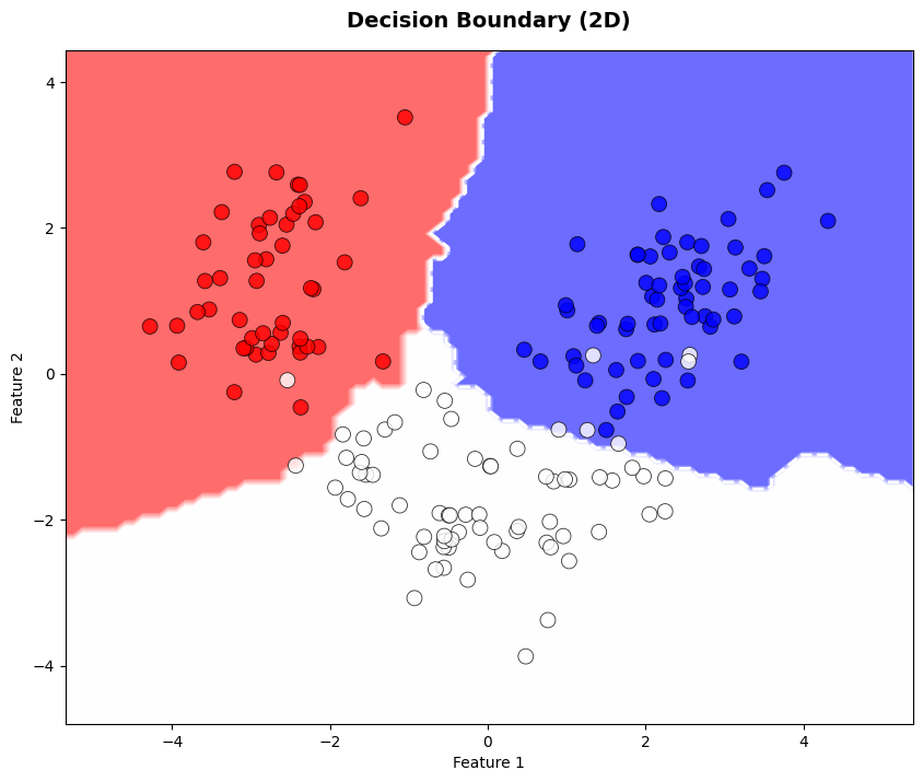
2D Matplotlib rendering |
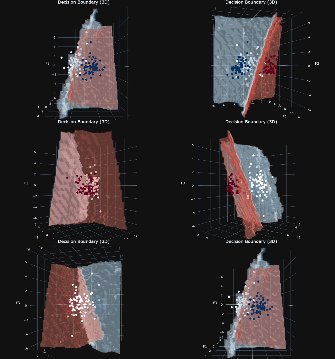
3D Interactive Plotly visualization |
Table of Contents
- About
- Interactive Examples & Tutorials
- How to Read the Plots
- Installation
- Quick Start & Basic Usage
- Dimensionality Reduction (N-D to 2D/3D)
- Live Training Callbacks
- How It Works Under the Hood
- Academic Use
About
Visualizing how a Machine Learning model partitions feature space is crucial for debugging, presentation, and deeply understanding model behavior. However, standard plotting libraries fail when your dataset has more than 2 or 3 features.
DecisionBoundary solves this by providing a universal visualization pipeline. It automatically handles high-dimensional data reduction, builds prediction grids, gracefully manages model interfaces (Scikit-Learn, Keras, PyTorch Lightning), and renders stunning 2D (Matplotlib) or 3D (Plotly) maps.
Key Features
| 🟢 Feature | Description |
|---|---|
| Universal Model Support | Works seamlessly with scikit-learn estimators, tf.keras neural networks, PyTorch Lightning modules, or any custom object with a .predict() method. |
| Auto Dimensionality Reduction | Natively supports PCA and UMAP. Pass 10D, 50D, or 100D data — the library automatically projects it down to 2D or 3D while preserving decision topographies using a built-in KNNInverseApproximator. |
| Live Training Callbacks | Watch your neural networks learn in real-time. Includes plug-and-play callbacks for Keras, Lightning, and Sklearn. |
| Dual Rendering Backends | High-performance static 2D plots via Matplotlib and fully interactive, rotatable 3D isosurfaces via Plotly. |
| Rich Customization | Effortlessly tweak colormaps, opacity, grid resolution, colorbars, and legend displays to make your charts presentation-ready. |
📘 Interactive Examples & Tutorials
Want to see it in action before writing code? Check out our interactive tutorials to explore basic plotting, styling, dimensionality reduction, and manual training loops:
- Google Colab: 👉 Run the DecisionBoundary Tutorial in the Cloud — Best for a quick, zero-setup interactive demo.
- Local Setup: Download the Tutorial Notebook (GitHub) — Best if you want to clone the repo, install dependencies locally, and play with your own datasets.
How to Read the Plots
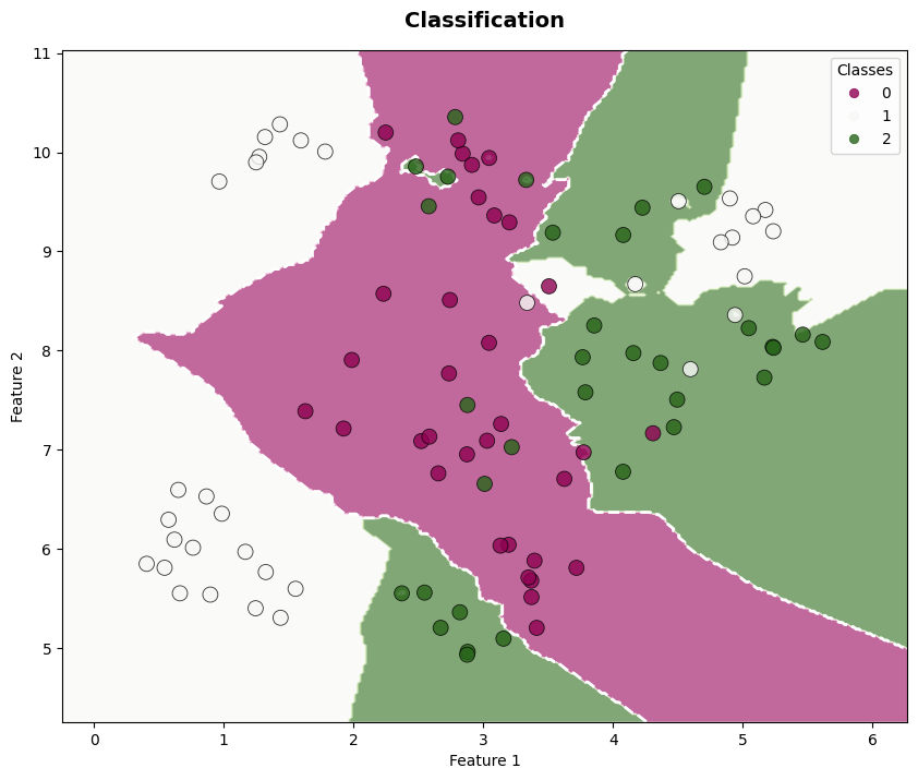
Discrete decision regions |
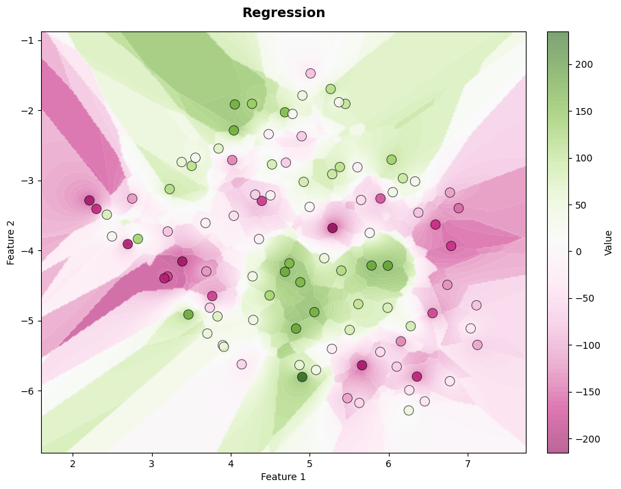
Continuous prediction surface |
When transitioning from native high-dimensional features to a reduced 2D/3D visual space, reading the boundary requires a specific intuition:
- The Background (Gradient/Surface): Represents the continuous prediction surface generated by your model across the compressed feature space.
- The Scatter Points: Represent the actual true labels ($y$) from your dataset.
Evaluating Model Quality: Ideally, the color of each individual scatter point should blend seamlessly with the background gradient directly beneath it.
⚠️ The Projection Caveat: If you see a stark contrast (e.g., a dark red point on a deep blue background), it usually indicates a model error. However, remember that you are looking at a compressed manifold. Points that are perfectly separated in 50D space might visually overlap when flattened to 2D. Always verify visual anomalies with your actual evaluation metrics (Accuracy, F1, RMSE)!
Installation
The core library is lightweight and easy to install via pip:
pip install decision-boundary-plot
Optional Dependencies: DecisionBoundary uses a modular dependency system to keep the core package light. Install extras based on your needs:
# Recommended for complex, non-linear dimensionality reduction
pip install decision-boundary-plot[umap]

# Required to save 3D interactive Plotly graphs as static .png files
pip install decision-boundary-plot[export]

# Required for the experimental Scikit-Learn 1.9.0+ callback support
pip install decision-boundary-plot[sklearn-callbacks]

# Install everything (includes sklearn callbacks, Keras, Lightning, UMAP, and Kaleido)
pip install decision-boundary-plot[all]
Alternatively, install the latest development version directly from GitHub:
# Install core development version (lightweight)
pip install git+https://github.com/P3Lin0r/decision-boundary.git

# Install development version with ALL extras (UMAP, Keras, Lightning, etc.)
pip install "decision-boundary-plot[all] @ git+https://github.com/P3Lin0r/decision-boundary.git"
Quick Start & Basic Usage
You don't need to manually create meshgrids, handle inverse transformations, or loop over predictions anymore. Just pass your data and a fitted model to the DecisionBoundary orchestrator.
The Basics (2D Classification)
from sklearn.datasets import make_classification
from sklearn.ensemble import RandomForestClassifier
from decision_boundary import DecisionBoundary

# 1. Prepare your data and fit a model
X, y = make_classification(n_features=5, n_informative=3, random_state=42)
model = RandomForestClassifier().fit(X, y)

# 2. Initialize the visualizer
# The library detects X has 5 dimensions and automatically applies PCA to reduce it to 2D
visualizer = DecisionBoundary(X, y, model=model, plot_mode="2d")

# 3. Render!
visualizer.plot(
    show=True,
    title="Random Forest Decision Boundary (5D -> 2D)",
    grid_resolution="normal"
)
Advanced Styling (kwargs)
The .plot() method accepts a rich set of styling arguments to make your charts presentation-ready. Whether you are doing classification or regression, you have full control over the aesthetics.
visualizer.plot(
    show=True,
    grid_resolution="high",       # "low", "normal", "high" or int (e.g., 200)

    # --- Aesthetics ---
    cmap="coolwarm",              # Colormap for the background gradient
    alpha=0.6,                    # Transparency of the background surface
    levels=100,                   # Number of contour levels (increase for smooth regression)

    # --- Toggles ---
    show_decision_line=False,     # Turn off the 0.5 threshold line (ideal for Regression)
    show_colorbar=True,           # Display a scale bar for continuous predictions
    show_legend=True,             # Display a discrete legend for classification targets

    # --- Labels ---
    colorbar_label="Predicted House Price ($)",
    legend_title="Iris Species",
    xlabel="Principal Component 1",
    ylabel="Principal Component 2",
)
💡 Tip: For a complete list of styling options, check out the
Plot2DKwargsandPlot3DKwargsdefinitions in the types source code.
Dimensionality Reduction (N-D to 2D/3D)
Real-world datasets rarely have just 2 or 3 features. When you pass high-dimensional data (e.g., 10D or 100D), DecisionBoundary seamlessly projects it down to a visualizable space.
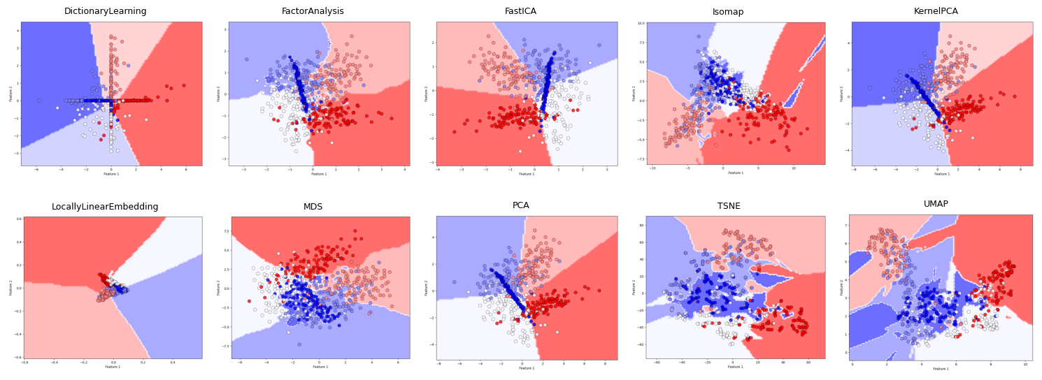
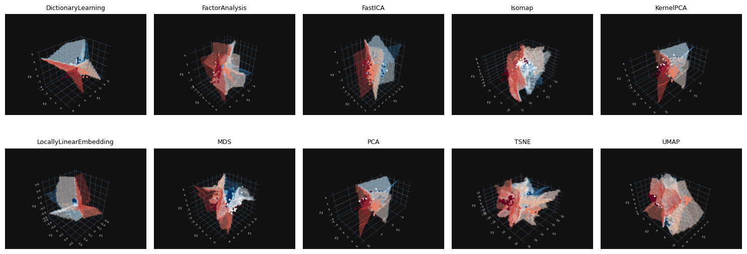
Comparing decision boundaries across different manifold learning algorithms.
Supported Algorithms
By default, the library uses dim_reducer="auto", which smartly selects PCA for highly linear/small datasets and UMAP for complex, non-linear manifolds.
You can explicitly force an algorithm or pass your own custom instantiated reducer (like t-SNE, Isomap, or any object exposing a .fit_transform() method):
from sklearn.manifold import TSNE

# 1. Using built-in string aliases: "pca", "umap", or "auto"
visualizer = DecisionBoundary(X, y, model, dim_reducer="umap")

# 2. Passing a custom configured instance
custom_tsne = TSNE(n_components=2, perplexity=15, random_state=42)

visualizer = DecisionBoundary(
    X, y, model,
    dim_reducer=custom_tsne,
    inverter_neighbors=15  # <--- Crucial for smooth backgrounds!
)
⚠️ The Inverse Transform Problem: To draw the background decision grid, the library must project 2D/3D screen coordinates back into original N-D space. Algorithms like PCA support this natively. Algorithms like t-SNE or Isomap do not. Solution: DecisionBoundary automatically injects a
KNNInverseApproximatorunder the hood. Use theinverter_neighborsparameter to control the smoothness of your background grid when using non-invertible reducers.
Live Training Callbacks (See your model learn!)
Static plots are great, but watching a model's decision boundary evolve epoch by epoch provides unparalleled intuition about its learning dynamics, overfitting, and activation function behaviors.

DecisionBoundary provides plug-and-play callbacks for the most popular ML/DL frameworks. All callbacks inherit from the same base class, meaning they share the exact same configuration parameters (plot_every, reuse, plotter_kwargs, save_dir, etc.). They can automatically save snapshots to disk or render them inline in Jupyter/Colab notebooks without violating any of your training logs.
💡 For more information about callback parameters, see the
BaseBoundaryCallback
🧠 Keras / TensorFlow
Seamlessly integrates with model.fit(). It even detects EarlyStopping to appropriately label your final "Best Model" plot!
from decision_boundary import KerasBoundaryCallback

callback = KerasBoundaryCallback(
    X_train, y_train,     # Tip: Pass validation X_val data for a more stable background representation
    plot_every=10,        # Render a plot every 10 epochs
    plot_mode="2d",       # Target dimension for the plot
    reuse=True            #
    reuse=True            # Update the same plot in Jupyter (prevents spam)
    save_dir="./plots",   # Automatically save plot in folder as PNG/HTML
    save_format="png",    # File format for saving the plot
)

model.fit(X_train, y_train, epochs=100, callbacks=[callback])
⚡ PyTorch Lightning
Monitors the Trainer lifecycle and triggers plot updates at the end of validation epochs.
from decision_boundary import LightningBoundaryCallback
import lightning.pytorch as pl

callback = LightningBoundaryCallback(X_train, y_train, plot_every=5)

trainer = pl.Trainer(max_epochs=50, callbacks=[callback])

trainer.fit(model, dataloader)
📊 Scikit-Learn (New in v1.9.0+)
The library actively supports the brand new experimental Callbacks API introduced in Scikit-Learn 1.9.0!
from sklearn.linear_model import LogisticRegression
from decision_boundary import SklearnBoundaryCallback

callback = SklearnBoundaryCallback(X_train, y_train, plot_every=5)

logreg = LogisticRegression(max_iter=100, solver='lbfgs')
logreg.set_callbacks(callback)
logreg.fit(X_train, y_train)
⚠️ Scikit-Learn Limitations: > As per the official sklearn documentation,
set_callbacksis currently only supported by models using thesolver='lbfgs'backend (e.g., Logistic Regression). Passing callbacks to other solvers will trigger a warning and be ignored by sklearn.
Custom Callbacks
Building your own training loop? Inherit from BaseBoundaryCallback to instantly get all the plotting orchestration, history caching, and file-saving logic for free!
How It Works Under the Hood
Curious about how DecisionBoundary elegantly maps a 100-dimensional neural network to a 2D screen? Here is the internal pipeline:
- Validation & Sampling (
validator.py): Checks inputs and safely downsamples massive datasets (e.g., 100k+ rows) via StratifiedSplit to maintain rendering performance without losing spatial distribution. - Adapter Pattern (
adapter.py): Wraps your model (whether it's Keras, Torch, or Sklearn) to standardize the.predict()outputs into a flat 1D float array, abstracting away probabilities, logits, or class indices. - Dimensionality Reduction (
reducer.py): Projects high-dimensional $X$ to 2D/3D. If the chosen algorithm lacks a nativeinverse_transform(like t-SNE), it seamlessly attaches theKNNInverseApproximatorto map screen coordinates back to the model's feature space. - Mesh Generation & Prediction (
renderer.py): Calculates an optimized coordinate grid, projects it to N-Dimensions, feeds it to the model, and builds the continuous probability surface. - Rendering (
renderer.py): Routes the resulting tensors to either thematplotlibbackend for static 2D or theplotlybackend for interactive 3D.
🎓 Academic Use
If you use this library for clustering analysis, computer vision research, or publish visualizations generated by DecisionBoundary in academic conferences, journals, or papers, please consider citing this repository:
@software{decision_boundary_2026,
  author = {Yermachenkov Illia},
  title = {Decision Boundary Visualizer: N-Dimensional ML Rendering},
  year = {2026},
  publisher = {GitHub},
  journal = {GitHub repository},
  url = {https://github.com/P3Lin0r/decision-boundary}
}
📄 License
Distributed under the MIT License. See LICENSE for more information. This means you are completely free to use this library in both open-source and closed-source commercial projects.
Enjoying the library? Drop a ⭐ on GitHub to show your support, it helps the project grow!
1 maintainer

Metadata
1 maintainer
Release files for decision-boundary-plot 0.1.0
For a detailed explanation of source distributions (sdists) and built distributions (wheels), please see the package formats documentation.
Source distribution (sdist)
| File | Size | Uploaded | |
|---|---|---|---|
| decision_boundary_plot-0.1.0.tar.gz | 49.0 kB | Details |
Built distribution (wheel)
| File | Interpreter | ABI | Platform | Reset |
|---|---|---|---|---|
| decision_boundary_plot-0.1.0-py3-none-any.whl | Python 3 | none | any | Details |
Total release size: 95.0 kB
Release files / decision_boundary_plot-0.1.0.tar.gz
| Download URL | decision_boundary_plot-0.1.0.tar.gz |
|---|---|
| Size | 49.0 kB |
| Tags | Source |
|
SHA-256 checksum How to use checksums |
78d14a88876247f01ba4adad2008217979f5cbfa46cc405c8cada4b4519d9dcd
|
|
BLAKE2b-256 checksum How to use checksums |
d51675126508043311e1aa9d277f731b9547c7f59983f01ffb0eb71cff7dc691
|
| Upload date | |
|
Uploaded using Trusted Publishing? What is trusted publishing? |
No |
| Uploaded via |
twine/6.2.0 CPython/3.14.6
|
Release files / decision_boundary_plot-0.1.0-py3-none-any.whl
| Download URL | decision_boundary_plot-0.1.0-py3-none-any.whl |
|---|---|
| Size | 46.0 kB |
| Tags | Python 3 |
|
SHA-256 checksum How to use checksums |
232ba0044d7f6b2d13114707c31d15874e5bd5ff5e82c5be706c44860ee023ae
|
|
BLAKE2b-256 checksum How to use checksums |
7cb839557a9ae4565c2b57e0ef327c47022f36a8b42997e16ba7715bb8228ca7
|
| Upload date | |
|
Uploaded using Trusted Publishing? What is trusted publishing? |
No |
| Uploaded via |
twine/6.2.0 CPython/3.14.6
|













