
DescriPyTor
Pick the atoms that matter, extract descriptors you can interpret, and find the model that explains your measurement.
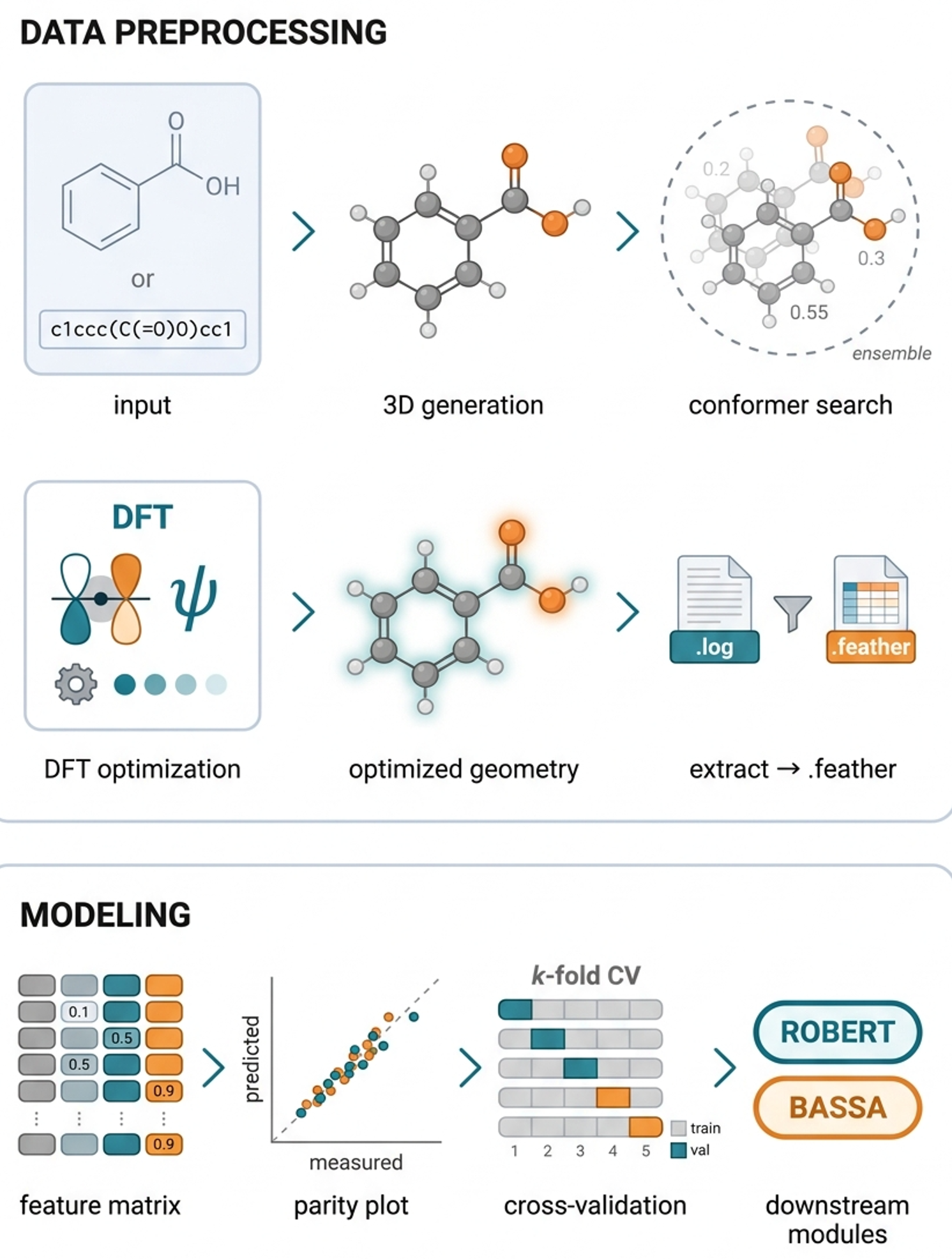
DescriPyTor turns quantum-chemistry output (Gaussian, ORCA, xTB) into a feature table that you define atom by atom, draws every descriptor on the molecule so you can see where a number comes from, and searches for the linear, classification or Bayesian model that fits the measured outcome.
Modeled after the R package MoleculaR (docs).
Structure in, descriptors out, model at the end.
Contents
- Install
- Five-minute tour
- The three pages
- Command line
- Python API
- Descriptors
- Modeling
- From SMILES on a cluster
- More tools
- Documentation
- Repository layout
Install
Python 3.9 to 3.11 (3.10 is what we test most). A conda environment is the easiest way to get RDKit.
conda create -n descripytor python=3.10 -y
conda activate descripytor
pip install descripytor
descripytor --help
From a clone (to change the code, run the tests, or use the case-study scripts):
git clone https://github.com/Milo-group/DescriPyTor.git
cd DescriPyTor
pip install -e ".[dev]"
pytest tests -q
Optional extras, added the same way (pip install "descripytor[bassa]", or pip install -e ".[bassa]" from a clone):
| Extra | Unlocks |
|---|---|
bassa |
bassa-reg, the spike-and-slab sampler behind new tables in the BASSA model explorer |
align |
torch, for MolAlign automatic atom renumbering |
engines |
mordred, deepchem, ase: extra descriptor engines |
explain |
SHAP model reports |
bayes |
pymc / arviz |
webapp |
the Streamlit extraction app |
If RDKit fails on pip: conda install -c conda-forge rdkit. numpy<2 is required. Gaussian, ORCA, xTB and Open Babel
are external programs and are not installed by pip. A Docker image with everything is described under More tools.
Five-minute tour
Everything below runs on data that ships with the package.
descripytor visual_extractor
- The page opens at http://127.0.0.1:7432 with an example molecule. Use example set points it at the bundled feathers; Apply example picks selects the atoms; Extract CSV computes the table for every molecule in the folder.
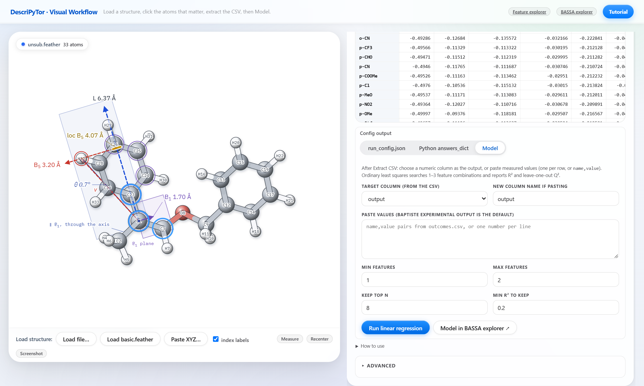
- In the Model tab, choose a target column or paste measured values, then either Run linear regression in the page, or
- Model in BASSA explorer ↗: one click sends the table, the target and the structures to the BASSA model explorer, which runs the sampler and shows the models beside the molecule.
Extracted table, measured outputs, and the two ways to model it.
The same three steps without a browser:
descripytor logs_to_feather                                        # Gaussian .log -> .feather (asks for the folder)
descripytor extractor -i input.json -o features -f feathers/       # the feature table
descripytor model -m regression -f features.csv -t targets.csv --min-features 2 --max-features 3
The three pages
Each page is one command, opens in the browser, and links to the other two in its header. All three draw molecules with the same engine, the feature explorer, so a descriptor looks the same wherever you meet it.
| Page | Command | What it is for |
|---|---|---|
| Visual extractor | descripytor visual_extractor |
pick atoms, extract the feature table for a folder, fit a quick model |
| Feature explorer | descripytor feature_explorer |
see any descriptor on the molecule, compare structures, make figures |
| BASSA model explorer | descripytor bassa_explorer |
read a Bayesian model search: which descriptors, in which models, on which compounds |
1. Visual extractor
descripytor visual_extractor                 # http://127.0.0.1:7432/visual
descripytor visual_extractor --port 8000 --no-browser
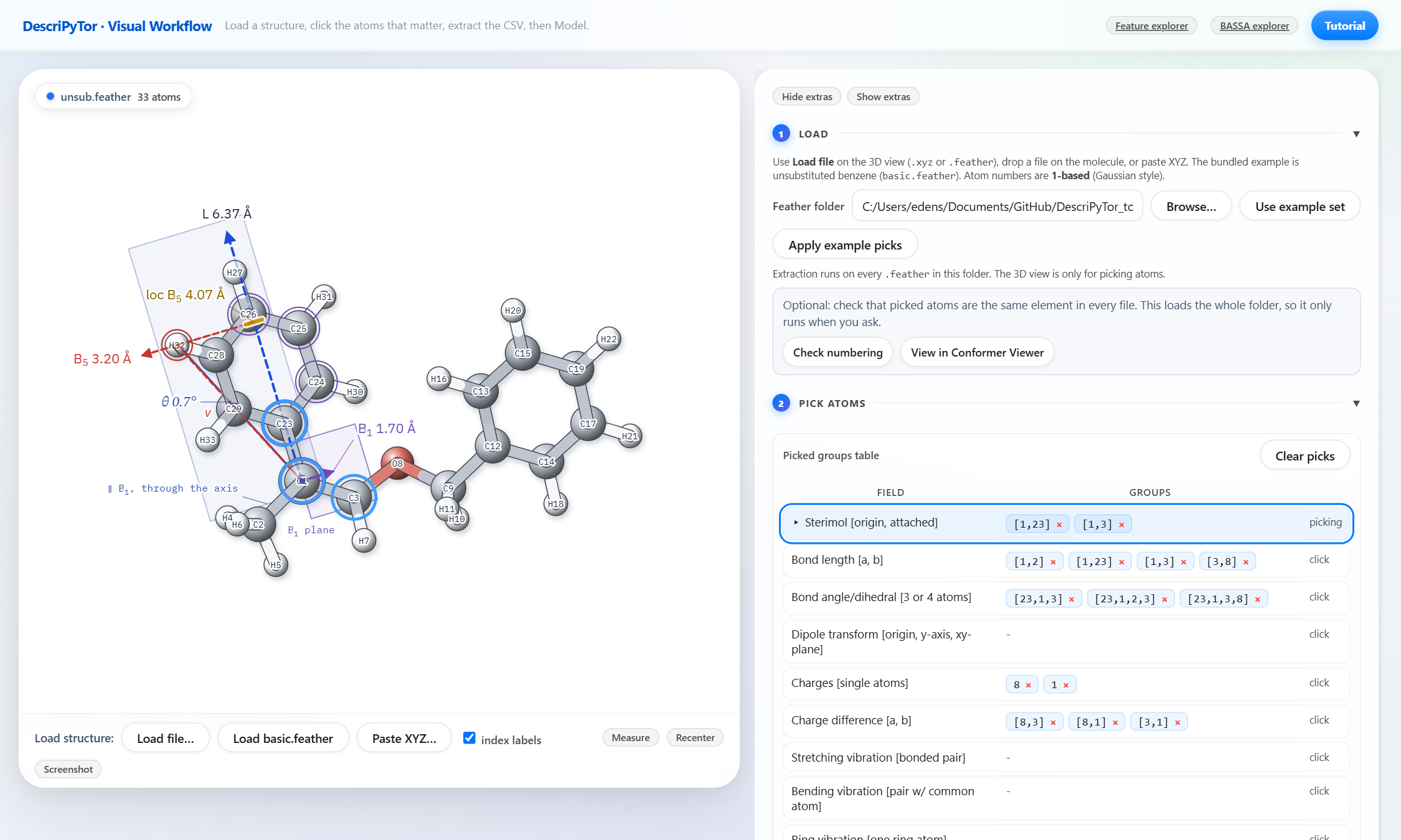
Load a .xyz or .feather (or drop it on the molecule), choose a descriptor field on the right, and click its atoms
in the figure. Pairs and triplets commit by themselves. Every selection is drawn as you make it: a Sterimol axis with
B1, B5, L and θ, the dipole in the frame you chose, a buried-volume sphere, and lengths, angles
and dihedrals with their values. Atom numbers are 1-based, as in Gaussian.
Pick a field, click atoms, see the construction and its value.
- Extract CSV runs the picks on every
.featherin the folder; Download CSV saves the table. - Save picks writes the input file that
descripytor extractorreplays on another set. - Check numbering confirms the picked atoms are the same element in every file.
- Model tab: linear regression in the page, or Model in BASSA explorer ↗.
- Further down the page: a conformer viewer that overlays an ensemble with RMSD, and a vibration-mode player.
- Tutorial (top right) is a five-step walkthrough.
2. Feature explorer
descripytor feature_explorer                                         # http://127.0.0.1:7432/feature_explorer
descripytor feature_explorer --mol FL_lig_13 --preset "theta construction"
Every construction on the molecule itself: the Sterimol axis, the B1 plane and its scan, loc B5, θ, cone angle, %Vbur, dipole frames, charges as sites or as a map, lengths and angles. Stack and superpose several structures, each with its own descriptors; lay panels out on a sheet; export SVG or PNG. The numbers are computed in the page by a line-for-line port of the Python, checked against it on every pick when the server is running.
The θ construction on a built-in structure.
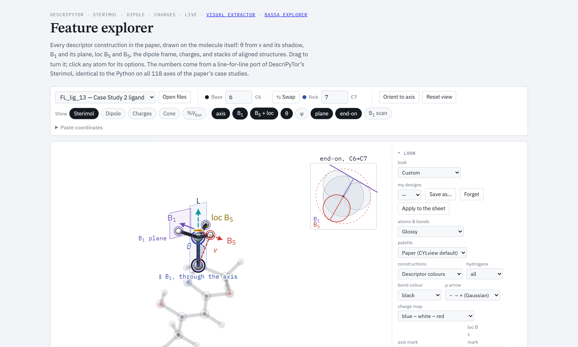
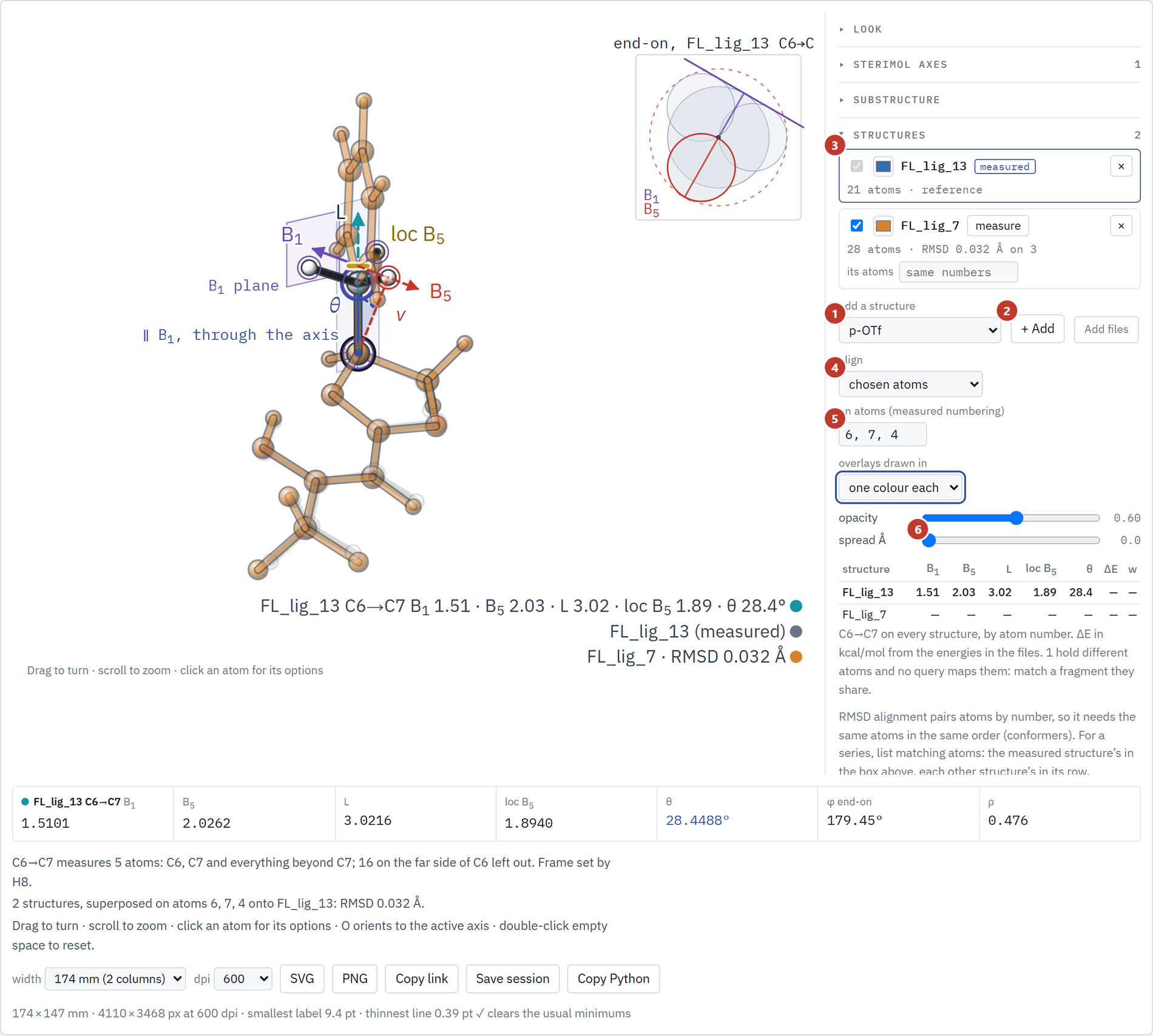
Left: stacked structures. Right: the B1 scan around the axis.
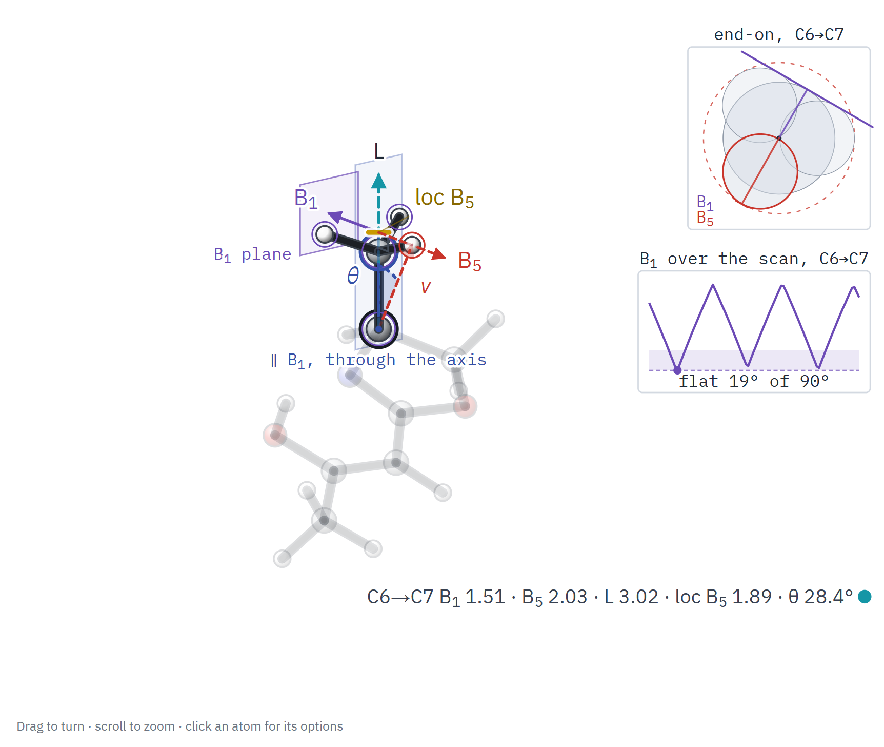
Open your own .xyz, .sdf, .feather or Gaussian .log with the file button; a feather or log brings the dipole
and the charges. A session (.featurescene.json) or an exported SVG reopens exactly as it was. Manual with every
control: docs/FEATURE_EXPLORER.md. Until October 2026 this page was called the Sterimol
theta explorer; descripytor theta and /theta still work.
3. BASSA model explorer
descripytor bassa_explorer                                   # http://127.0.0.1:8765, opens a bundled example
descripytor bassa_explorer --cases my_cases --bassa-python C:/envs/bassa/python.exe
BASSA is a spike-and-slab sampler: instead of one winning equation it visits many models and reports how often each descriptor is in them. The page puts that run beside the molecule. Columns are the models visited, rows are descriptors, and the feature explorer on the right draws the descriptors of the selected model on any compound.
The run handed over from the visual extractor: 18 compounds, 43 descriptors.
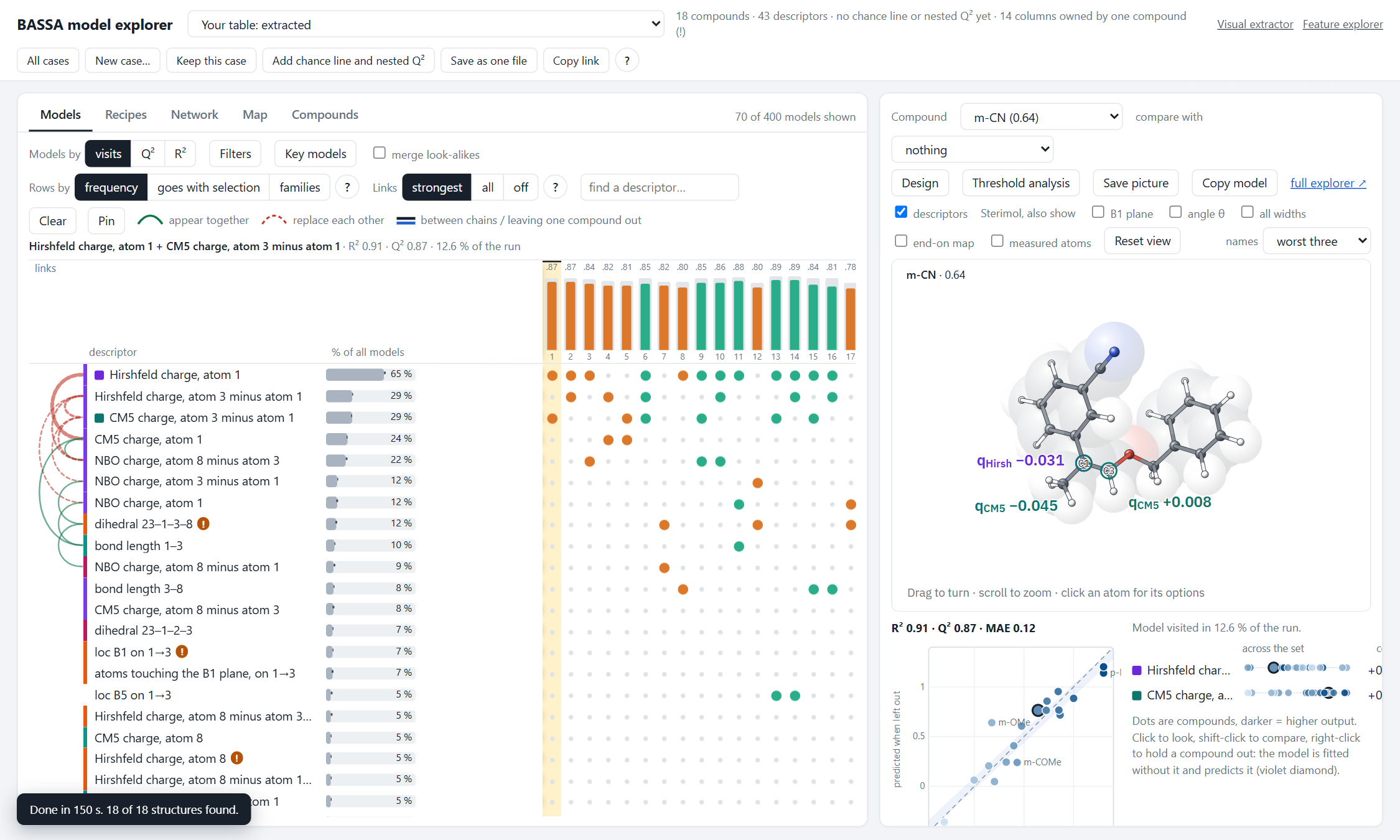
- New case… takes a CSV (first column the compound name, one response column, the rest descriptors) and,
optionally, a folder of
.feather,.logor.xyzfiles named like the compounds. Or arrive from the visual extractor with one click. - Add chance line and nested Q² reruns the sampler on 100 shuffles of the response and once per compound left out.
- Keep this case stores it in the cases folder (
--cases, default./bassa_cases); Save as one file writes a single HTML that opens without a server. - Shift-click compounds in the plot to stack them, each with its own values.
Running a new table needs the sampler: pip install "descripytor[bassa]", or point --bassa-python (or the
environment variable DESCRIPYTOR_BASSA_PYTHON) at a Python that has bassa-reg. Without it the page still opens the
example and every kept case. The corrected sampler core is the default: the released bassa-reg core is wrong
when descriptors are correlated, and the package runs its own corrected copy
(M3_modeler/bassa_explorer/core_fixed.py). BASSA_CORE=package runs the released one instead.
Manual: docs/BASSA_EXPLORER.md.
Command line
descripytor <command> [options]            descripytor --help            descripytor <command> --help

Pages
  visual_extractor   pick atoms on a molecule, extract descriptors for a folder, fit a model      (alias: visual)
  feature_explorer   draw any descriptor on the molecule                                           (alias: theta)
  bassa_explorer     the models a BASSA run visited, beside the molecule                           (alias: bassa)

Batch
  extractor          descriptors for a folder of .feather files, from an input file of atom choices
  model              search regression or classification models over a feature table
  pipeline           SMILES -> structures -> chained cluster stages (GOAT / UMA / xTB / ORCA / Gaussian)

Converters (they ask for their inputs)
  logs_to_feather    Gaussian .log files -> .feather
  sterimol           Sterimol from .xyz files
  cube               Sterimol from Gaussian cube files
| Command | Options |
|---|---|
visual_extractor |
--port (7432), --host, --no-browser |
feature_explorer |
--mol NAME, --preset NAME, --port, --host, --no-browser |
bassa_explorer |
--cases DIR, --bassa-python PYTHON, --port (8765), --host, --no-browser |
extractor |
-i input.json, -o output_name, -f feather_dir |
model |
-m {regression,classification}, -f features.csv, -t targets.csv, -y name, -j cores, --min-features, --max-features, --top-n, --threshold, --leave-out, --bool-parallel |
pipeline |
{build,adopt,submit,status,retry,reset,watch,fetch} protocol.json and its flags (docs/PIPELINE.md) |
Examples:
# descriptors for the bundled benzenes, from the bundled atom choices
descripytor extractor -i descripytor/examples/feather_example/input_example.json \
                      -o feature_set -f descripytor/examples/feather_example

# every 1- to 3-descriptor linear model, the best 20 kept, on all cores
descripytor model -m regression -f features.csv -t targets.csv -y output \
                  --min-features 1 --max-features 3 --top-n 20 --threshold 0.7 --bool-parallel -j -1

# classification, two samples held out for external validation
descripytor model -m classification -f features.csv -t labels.csv --leave-out L3 L12
Python API
Extract a feature table and search models, on the bundled set of 18 substrates with measured outputs:
from M2_data_extractor.data_extractor import Molecules
from M3_modeler.modeling import LinearRegressionModel
from descripytor.examples import baptiste_example_dir

folder = baptiste_example_dir()
mols = Molecules(str(folder))                     # every .feather in the folder
features = mols.get_molecules_features_set({
    "Dipole": "23,24,25,26,27,28,23,1",           # origin atoms (ring centroid), y-axis atom, plane atom
    "Charges": "8,1",
    "Charge difference": "8,3 8,1 3,1",
    "Sterimol": "1,23 1,3",
    "Bond length": "1,2 1,23 1,3 3,8",
    "Bond angle": "23,1,3 23,1,2,3",              # three atoms: angle; four: dihedral
})
features.to_csv("features.csv")

model = LinearRegressionModel(
    {"features_csv_filepath": "features.csv",
     "target_csv_filepath": str(folder / "outcomes.csv")},
    process_method="two csvs", y_value="output",
    min_features_num=2, max_features_num=2)
top = model.search_models(top_n=5, threshold=0.5)   # prints the ranked models, then asks which one to plot
One molecule, one descriptor at a time:
mol = mols.molecules[0]
mol.get_sterimol([1, 23])                        # B1, B5, L, loc_B1, loc_B5, B1_B5_angle (theta), ...
mol.get_dipole_gaussian_df([[23, 24, 25, 26, 27, 28], 23, 1])
mol.get_charge_df([8, 1])                        # every charge type in the file
mol.get_bond_angle([[23, 1, 3], [23, 1, 2, 3]])
mol.get_stretch_vibration([1, 2])                # the pair must be bonded
mol.get_ring_vibrations([23])                    # one ring atom; ortho / meta / para are found
mols.get_sterimol_dict([[1, 23], [1, 3]])        # the same for every molecule, as one table
Metal complexes, from a single structure or a conformer ensemble (docs/METAL_COMPLEX.md):
from M2_data_extractor.metal_complex import MetalComplex, MetalComplexEnsemble

geo = MetalComplex.from_xyz("026_lig_CuCl.xyz").geometric_features()
# fromM_* : Sterimol read from the metal; sub_* : from the stereocentre; bite, M-D distances, %Vbur, ...
ens = MetalComplexEnsemble.from_xyz("081_lig.finalensemble.xyz").geometric_features()   # Boltzmann-averaged
Exhaustive search with honest validation (docs/WORKFLOW.md):
from M3_modeler.ridge_search import all_combos, loo_predictions, adj_q2, nested_loo
from M3_modeler.validation import selection_null

combos = all_combos(X.shape[1], 3)
pred = loo_predictions(X, y, combos, lam=1.0)     # lam=0: ordinary least squares
best = combos[adj_q2(pred, y, 3).argmax()]
nested = nested_loo(X, y, combos)                 # re-select inside every leave-one-out fold
null = selection_null(X, y, combos, lam=0, n_perm=1000)   # the whole search on permuted y: null["p"]
Class reference: M2_data_extractor/README.md and M3_modeler/README.md.
Descriptors
Most descriptor packages return thousands of columns. DescriPyTor asks which atoms matter and returns a few descriptors you already understand, each read in a frame you define.
Trim by symmetry, align to a shared frame, pick the descriptors that mean something.
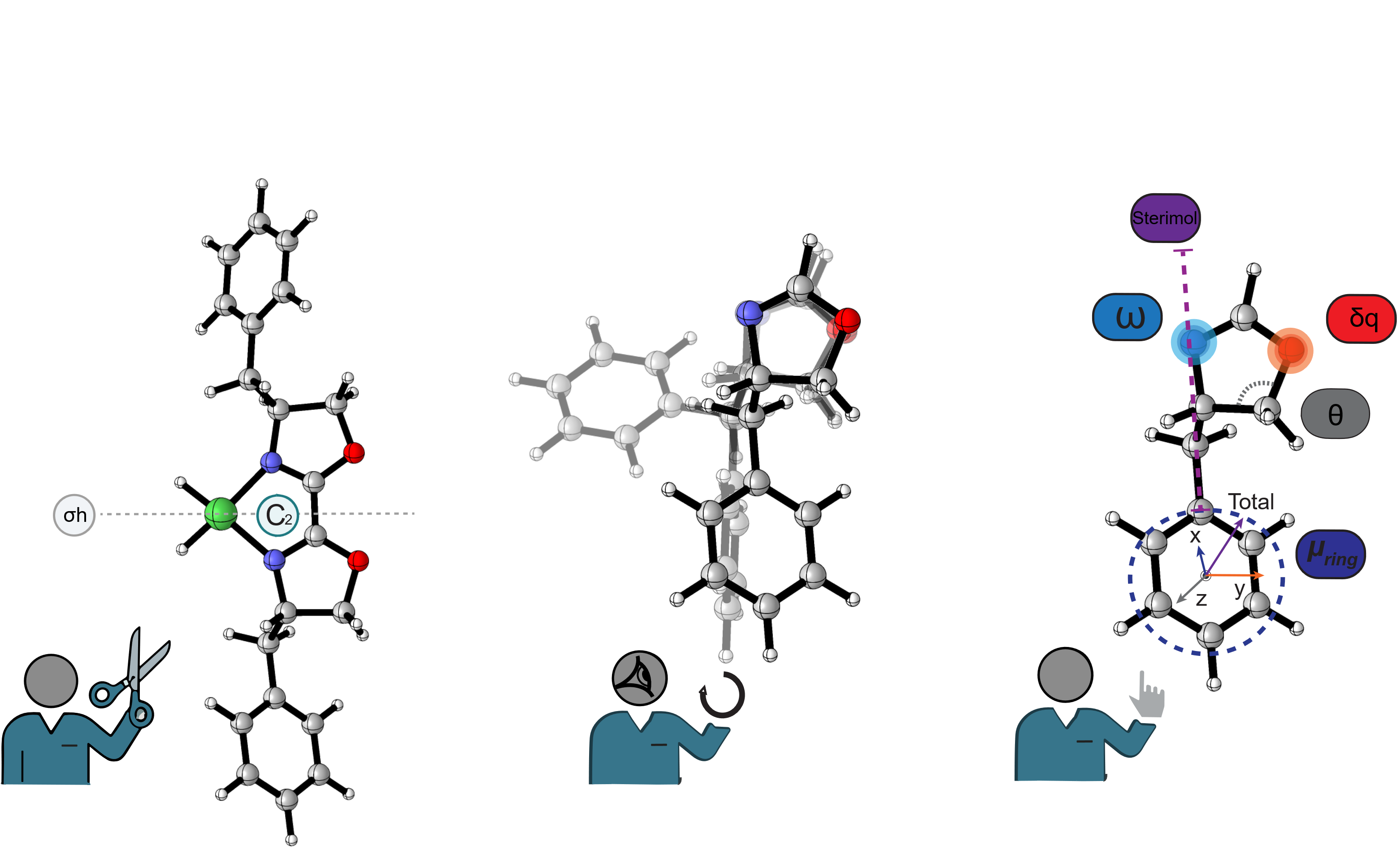
| Family | What you give it | What you get |
|---|---|---|
| Sterimol | [origin, attached] atom pair |
L, B1, B5, where along the axis they sit (loc_B1, loc_B5), and θ, the angle between B1 and B5 |
| Cube Sterimol | a density .cube file |
Sterimol from the electron density instead of tabulated radii |
| Charges | single atoms | NBO / Hirshfeld / CM5 values per atom |
| Charge difference | atom pair [a, b] |
q_a − q_b, per charge scheme |
| Dipole | [origin(s), y-axis, xy-plane] |
dipole components in your frame, and the total |
| Bond length / angle | pairs, triads or quartets | distances, angles, dihedrals |
| Stretching vibration | a bonded pair | frequency and amplitude of the mode along that bond |
| Bending vibration | two atoms sharing a centre | frequency and amplitude of the bending mode |
| Ring vibration | one ring atom | cross / para frequencies and angles of the ring |
| Buried volume, cone angle, SASA, dispersion | metal or apex atom | via morfeus |
| Metal complex | complex XYZ, optional xTB output | fromM_*, sub_*, %Vbur, charges, bond orders, graph indices |
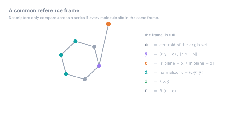
A common frame. Every molecule is rotated onto the same origin and axes, so "the dipole along y" means the same thing in every row. You pick three groups: the origin is their centroid, ŷ points at the y-atom, and x̂ is the plane atom with its ŷ part removed.
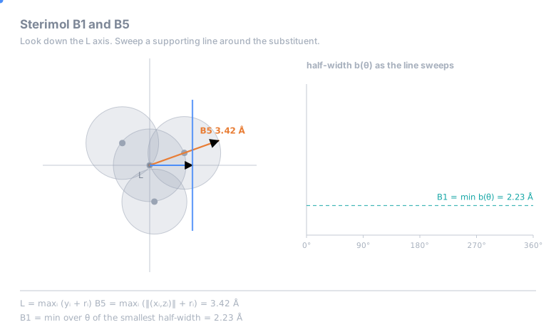
Sterimol. L runs along the chosen bond; B5 is the furthest reach from the axis; B1 is the smallest width,
found by turning a tangent line all the way round the group.
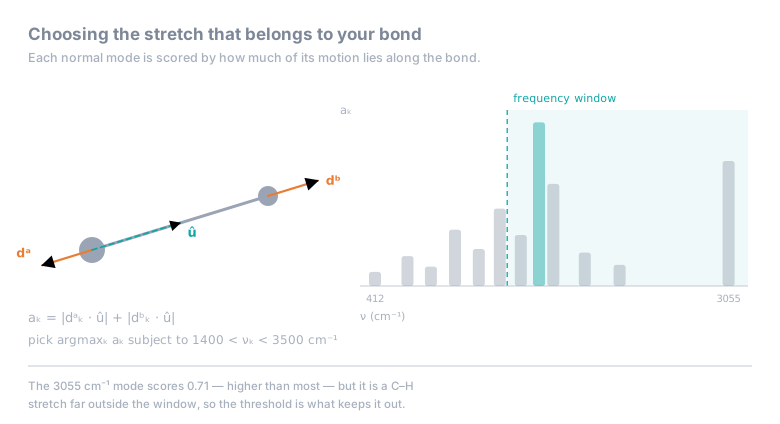
Vibrations. Each normal mode is scored by how much of its motion lies on the atoms you named; the best score inside a frequency window is taken. Keep the window tight, or a C–H stretch can beat your carbonyl.
What to decide and check at each step of an extraction: docs/EXTRACTION_PROTOCOL.md. What changed in the descriptor definitions, and why: docs/STERIMOL_FIXES.md, docs/FEATURE_FIXES.md.
Modeling
Three ways, from quick to thorough:
| Where | What it does | |
|---|---|---|
| Linear regression in the page | visual extractor, Model tab | every 1- to 3-descriptor model, R² and leave-one-out Q² |
| Exhaustive search with a report | descripytor model, M3_modeler |
regression or classification over every subset, scaling inside each fold, a PDF report |
| Bayesian model averaging | descripytor bassa_explorer |
inclusion frequency of every descriptor over the models the sampler visits |
descripytor model -m regression -f features.csv -t targets.csv -y output \
                  --min-features 1 --max-features 4 --top-n 20 --threshold 0.70 --bool-parallel -j -1
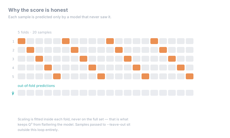
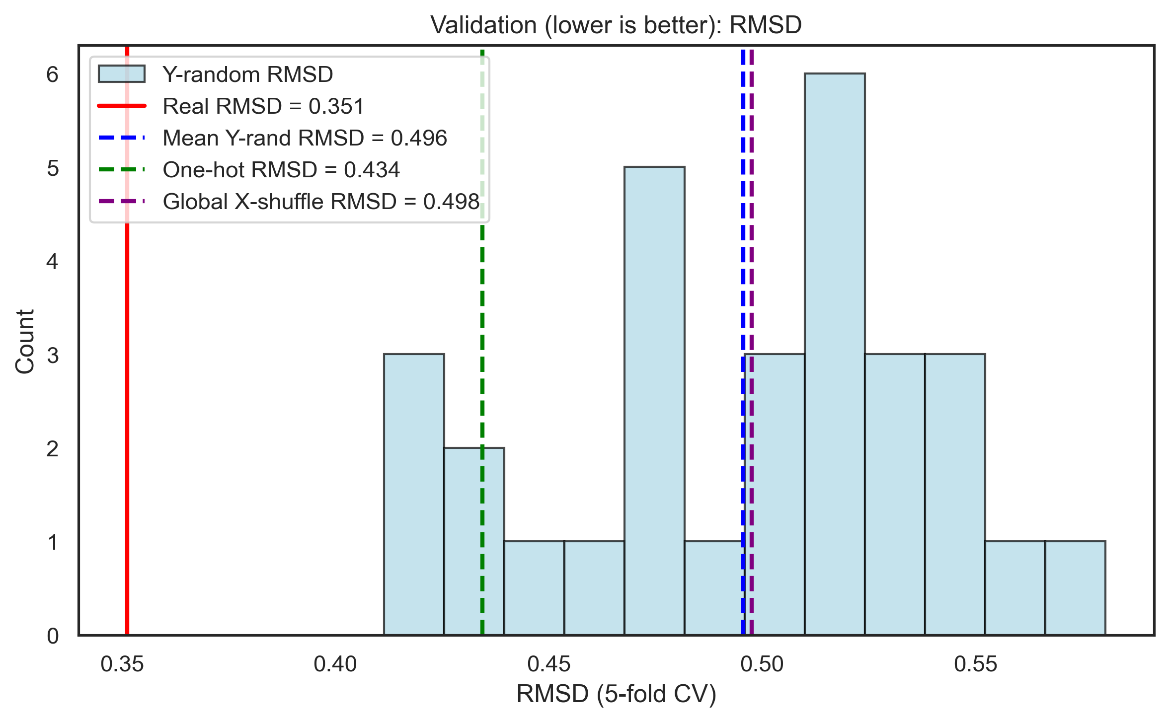
With few molecules and many subsets, R² can look fine and mean nothing. Q² uses only predictions for samples the model never saw; that is the number to read. The report also refits against shuffled targets, shuffled descriptors and a one-hot baseline: a real model has to beat all of them.
The real model sits clear of the shuffled-target distribution. Inside it, the model is fitting noise.
runs/<dataset>_<target>_<date>/
  db/    every model scored (CSV and SQLite), so reruns are incremental
  figs/  coefficients, parity, SHAP, sanity checks, diagnostics
  pdf/   <dataset>_top_models_report.pdf
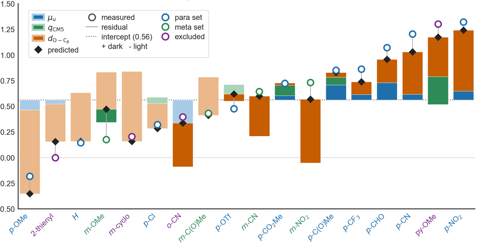
Per-compound breakdown: which descriptor moved which prediction, and by how much.
From SMILES on a cluster
descripytor pipeline takes a table of SMILES to numbered structures and chains conformer search and
quantum-chemistry stages (GOAT, UMA, xTB, ORCA, Gaussian) on an SGE cluster, one action at a time:
descripytor pipeline build  protocol.json        # SMILES -> numbered xyz
descripytor pipeline submit protocol.json --dry-run
descripytor pipeline status protocol.json
descripytor pipeline fetch  protocol.json
Protocol format and every flag: docs/PIPELINE.md.
More tools
-
Atom renumbering (
MolAlign/): matches atom numbering across a series so descriptors line up. Needstorch(pip install -e ".[align]"), thenpython MolAlign/renumbering.py --help. -
Other descriptor engines in one pass (RDKit, Mordred, DeepChem, morfeus, AQME/xTB), merged into one CSV: descriptor_extraction_toolkit/README.md.
-
Old definitions on request:
with descripytor.compat.paper_v3(): ...computes with the definitions of the paper's tag. -
Docker (RDKit, morfeus, AQME, Mordred and xTB preinstalled):
docker compose up --build # pages on http://localhost:7432, files in work/ (mounted at /work)
Setup from scratch: DOCKER_QUICKSTART.md.
Documentation
| QUICKSTART.md | one page: install and first run |
| docs/WORKFLOW.md | logs → features → model → validation, with every option |
| docs/EXTRACTION_PROTOCOL.md | what to decide and check at each step of an extraction |
| docs/FEATURE_EXPLORER.md | the feature explorer, control by control, with screenshots |
| docs/BASSA_EXPLORER.md | the BASSA model explorer: starting it, your own table, reading a case |
| docs/METAL_COMPLEX.md | descriptors of metal complexes from GOAT / xTB output |
| docs/PIPELINE.md | the cluster pipeline |
| docs/visual-guide.md | a visual handout for a first session |
| Getting_started_with_examples/ | notebooks for extraction and modeling, example data |
| CHANGELOG.md | what changed, release by release |
Bundled data: 10 substituted benzenes (descripytor.examples.feather_example_dir()), 18 substrates with measured
outputs (descripytor.examples.baptiste_example_dir()), ready-made linear and logistic datasets
(Getting_started_with_examples/modeling_example/), and density cubes for cube Sterimol.
Repository layout
descripytor/                    the installable package: the command line, examples, compat.paper_v3()
M1_pre_calculations/            structures and calculation inputs; pipeline/ (the cluster pipeline)
M2_data_extractor/              descriptor extraction: Molecules, Molecule, MetalComplex
  atom_picker.html                the visual extractor's page, served by gui_server.py
  feature_explorer/               the feature explorer: sources, build.py, and the gates that check it against the Python
M3_modeler/                     model search, ridge_search, validation
  bassa_explorer/                 the BASSA model explorer: page, server, sampler set-up, a bundled example
MolAlign/                       alignment and atom renumbering
utils/                          shared file handling, geometry, visualization
Getting_started_with_examples/  notebooks, example data, the multi-engine toolkit
docs/                           manuals, images, animations
tests/                          pytest suite and its data
Atom indices are 1-based everywhere, matching Gaussian. The pictures of this page are regenerated by
docs/images/readme/make_images.py, the animations by docs/animations/build_animations.py.
License
MIT. See LICENSE.
1 maintainer

Metadata
1 maintainer
Release files for descripytor 0.3.1
For a detailed explanation of source distributions (sdists) and built distributions (wheels), please see the package formats documentation.
Source distribution (sdist)
| File | Size | Uploaded | |
|---|---|---|---|
| descripytor-0.3.1.tar.gz | 5.1 MB | Details |
Built distribution (wheel)
| File | Interpreter | ABI | Platform | Reset |
|---|---|---|---|---|
| descripytor-0.3.1-py3-none-any.whl | Python 3 | none | any | Details |
Total release size: 10.3 MB
Release files / descripytor-0.3.1.tar.gz
| Download URL | descripytor-0.3.1.tar.gz |
|---|---|
| Size | 5.1 MB |
| Tags | Source |
|
SHA-256 checksum How to use checksums |
4f6d4b9fd55ba3c35c440aae287486204cd74d6eaa30bfec5ce74effb3166eab
|
|
BLAKE2b-256 checksum How to use checksums |
6910c756304d019db542a256828a8b985f7cd2ed59bd8cc8453afb7947ab4a1c
|
| Upload date | |
|
Uploaded using Trusted Publishing? What is trusted publishing? |
No |
| Uploaded via |
twine/7.0.0 CPython/3.11.5
|
Release files / descripytor-0.3.1-py3-none-any.whl
| Download URL | descripytor-0.3.1-py3-none-any.whl |
|---|---|
| Size | 5.2 MB |
| Tags | Python 3 |
|
SHA-256 checksum How to use checksums |
81586126c8ff82726958ffbd43141fe1b37b07e0cc9fe622fc97e2dfc08539e5
|
|
BLAKE2b-256 checksum How to use checksums |
191679586076615ef4f75ebc6a7fad0149025c743d9f7eeafaf746bc3d29a0be
|
| Upload date | |
|
Uploaded using Trusted Publishing? What is trusted publishing? |
No |
| Uploaded via |
twine/7.0.0 CPython/3.11.5
|














