
dfm-python





Linear, deep and attention-based dynamic factor models in Python, behind one scikit-learn-style estimator API.
| Model | What it is | Backend |
|---|---|---|
DFM |
linear, mixed-frequency dynamic factor model, estimated by EM with Kalman filtering and smoothing | numpy |
DDFM |
deep dynamic factor model: a nonlinear encoder trained with MCMC denoising and a linear state space on its factors | PyTorch |
iVDFM |
identifiable variational dynamic factor model, trained on the ELBO with a context-conditioned innovation prior | PyTorch |
AFM |
Attention Factor Model of Epstein, Wang, Choi and Pelger (2025): a cross-sectional conditional factor model whose residuals are traded portfolios, with PCA and Avellaneda-Lee benchmarks | PyTorch |
Contents: Why dfm-python · Installation · Quick start · Estimator API · Models · Data · Saving and loading · YAML configurations · Migrating from 0.7 · Known limitations · Development · Security · Citing · Star history
Why dfm-python
- Mixed-frequency DFM on any clock. The latent factors evolve at one
clock frequency (daily, weekly, monthly, quarterly, semiannual or annual),
and series sampled at one slower frequency load on them through a tent
kernel you choose, for example
{"q:m": [1, 2, 3, 2, 1]}for quarterly series on a monthly clock. Columns can be in any order. - An exact Kalman filter and EM, checked against independent references.
The E-step is an in-house float64 Kalman filter and Durbin-Koopman smoother
that uses every observed entry (missing values are handled per element);
the M-step is the closed-form Banbura-Modugno (2014) update;
loglikis the exact Gaussian log-likelihood at the returned parameters. The test suite checks the E-step, EM monotonicity and the M-step against a reference Kalman filter that does not import the package, and against statsmodels'KalmanSmootherwhen it is installed. - Deep and identifiable factor models on the same API. DDFM (nonlinear encoder, MCMC denoising) and iVDFM (variational, identifiable through a context-conditioned innovation prior) fit, forecast, update and save exactly like the linear DFM, on CPU or GPU.
- An attention factor model for statistical arbitrage. AFM learns conditional factors from firm characteristics and a trading policy on the residual portfolios under an after-cost Sharpe objective, with the PCA + LongConv and PCA + Avellaneda-Lee benchmarks behind two switches.
- One scikit-learn-style API. Hyperparameters in the constructor,
fit(data)on onePanelDatacontainer, DataFrame forecasts in data units and in your column order, fitted state in attributes ending in_,get_params/set_params/sklearn.base.clone, andupdate(data)to condition on new observations without refitting. - Pickle-free save directories and YAML configs.
save(path)writes JSON,.npzand (for torch models) aweights_onlystate dict thatdfm_python.load(path)reads back without data, on any device. A YAML file withmodel:anddata:sections builds exactly the constructor call and thePanelData; unknown keys raise.
How the linear DFM compares with statsmodels' DynamicFactorMQ (statsmodels
0.15), which implements the same Banbura-Modugno EM:
statsmodels DynamicFactorMQ |
dfm-python DFM |
|
|---|---|---|
| Mixed frequencies | monthly with quarterly | any clock (d, w, m, q, sa, a) with one slower frequency |
| Aggregation weights | fixed [1, 2, 3, 2, 1] |
the tent kernel you pass in tent_weights |
| Data layout | quarterly series in endog_quarterly, or after the monthly ones with k_endog_monthly |
any column order; frequencies in PanelData.freq |
| News decomposition | news() |
not available |
| Nonlinear models on the same API | no | DDFM, iVDFM, AFM |
Installation
pip install dfm-python # or: uv add dfm-python
dfm-python supports Python 3.10 to 3.13. The runtime dependencies are numpy,
pandas, scipy, scikit-learn, torch (2.10 or newer) and einops. PyTorch is a required
dependency even if you only use the numpy DFM, because the package imports
it. pip installs the default PyTorch wheel for your platform; for a CPU-only
or a specific CUDA build, install torch first from the
PyTorch index, for example
pip install torch --index-url https://download.pytorch.org/whl/cpu, then
install dfm-python. The torch models take device="auto" (CUDA when
available, else CPU), a device string such as "cpu" or "cuda:0", or a torch.device.
Optional extras:
| Extra | Adds | Needed for |
|---|---|---|
yaml |
omegaconf | YAML configs (load_yaml, XConfig.from_yaml) and the tutorial/ scripts |
tune |
optuna | iVDFM hyperparameter search (dfm_python.tuning) |
metrics |
sktime | calculate_rmse, calculate_mae |
polars |
polars, pyarrow | passing polars DataFrames to PanelData |
all |
all of the above | |
dev |
pytest, pytest-cov, ruff, build, twine, omegaconf, pyyaml, optuna, statsmodels | running the test suite and building the package |
pip install "dfm-python[yaml,tune]"
Without an extra, the code that needs it raises an ImportError naming the
extra to install. PyYAML also works for load_yaml.
Quick start
A one-factor, mixed-frequency DFM: three monthly indicators and quarterly GDP growth on a monthly clock. It runs in a few seconds on a laptop.
import numpy as np
import pandas as pd
from dfm_python import DFM, PanelData

# Ten years of monthly data driven by one AR(1) factor: three monthly
# indicators and quarterly GDP growth (observed in Mar, Jun, Sep, Dec).
rng = np.random.default_rng(0)
f = np.zeros(120)
for t in range(1, 120):
    f[t] = 0.8 * f[t - 1] + rng.standard_normal()
idx = pd.date_range("2015-01-31", periods=120, freq="ME", name="date")
df = pd.DataFrame({"ip": f, "sales": 0.7 * f, "jobs": -0.5 * f}, index=idx)
df += 0.5 * rng.standard_normal(df.shape)
df["gdp"] = np.convolve(f, [1, 2, 3, 2, 1])[:120] / 9   # tent-weighted monthly factor
df.loc[df.index.month % 3 != 0, "gdp"] = np.nan          # quarterly: NaN between releases

data = PanelData(y=df, freq={"gdp": "q"})                # unlisted series run at the clock
model = DFM(n_factors=1, clock="m", tent_weights={"q:m": [1, 2, 3, 2, 1]},
            scaler="standard", max_iter=100).fit(data)

model.result_.loglik, model.n_iter_, model.converged_    # exact log-likelihood, EM diagnostics
fc = model.predict(6)               # DataFrame 6 x 4: every series at every month, in data units
zf = model.predict_factors(6)       # DataFrame 6 x state dimension (state_0, ...)
model.save("runs/quickstart", overwrite=True)            # pickle-free directory
The Models section has a
complete example for each model, and
tutorial/
fits each of DFM, DDFM and iVDFM to the three shipped datasets.
The estimator API
Every model follows the same contract, modelled on scikit-learn:
Model(**hyperparameters)stores keyword-only hyperparameters and does nothing else.fit(data)takes aPanelData(or a DataFrame) and returns the model.predict(h)returns a DataFrame of thehsteps after the last conditioning date, one column per series in your order, in data units.predict_factors(h)returns the factor (state) forecast. AFM allocates instead:allocate()andbacktest(data).- Fitted state lives in attributes ending in
_:result_,n_iter_,converged_,scaler_,factors_, ... Beforefitthey raiseNotFittedError. update(data)conditions later forecasts on new data with the fitted parameters;update(data, refit=True)also re-estimates where the model supports it.save(path)writes a pickle-free directory;Model.load(path)anddfm_python.load(path)read it back without data.get_params,set_paramsandsklearn.base.clonework as in scikit-learn, andget_config()/Model.from_config(cfg)convert to and from the typed config mirror (DFMConfig,DDFMConfig,iVDFMConfig,AFMConfig).
import numpy as np
import pandas as pd
from sklearn.base import clone

import dfm_python
from dfm_python import DFM, PanelData

idx = pd.date_range("2015-01-31", periods=96, freq="ME", name="date")
df = pd.DataFrame(np.random.default_rng(0).standard_normal((96, 3)),
                  index=idx, columns=["a", "b", "c"])
train, new = PanelData(y=df.iloc[:84]), PanelData(y=df.iloc[84:])

model = DFM(n_factors=1, max_iter=50, scaler="standard")  # hyperparameters only
model = model.fit(train)                                  # fit returns the model
fc = model.predict(6)               # DataFrame 6 x 3, index 2022-01-31 ... 2022-06-30
zf = model.predict_factors(6)       # DataFrame 6 x state dimension (state_0, ...)
model.result_.loglik, model.n_iter_, model.converged_

model.update(new)                   # condition on the 12 new rows; returns model
assert model.predict(6).index[0] == pd.Timestamp("2023-01-31")

model.save("runs/quickstart", overwrite=True)            # pickle-free directory
same = dfm_python.load("runs/quickstart")                # or DFM.load(...); no data needed
pd.testing.assert_frame_equal(same.predict(6), model.predict(6))

params = model.get_params()                              # {"n_factors": 1, ...}
two = clone(model).set_params(n_factors=2)               # unfitted copy with 2 factors
cfg = model.get_config()                                 # DFMConfig with the same fields
assert DFM.from_config(cfg).get_params() == params
The public names are exported from dfm_python: the models DFM, DDFM,
iVDFM, AFM (and their base BaseFactorModel), the configs DFMConfig,
DDFMConfig, iVDFMConfig, AFMConfig, PanelData, load, the results
BaseResult, DFMResult, DDFMResult, calculate_rmse, the errors
NotFittedError and UnsupportedInputError, and set_verbosity /
get_verbosity.
Models
Each model's full parameter list is in its docstring (help(DFM)); the
tables below list the main hyperparameters with their defaults.
DFM
DFM, the linear dynamic factor model, is estimated by EM with Kalman
filtering and smoothing. The series are PanelData.y, in any column order,
and their frequencies PanelData.freq. The latent factors evolve at the
clock frequency. Every series is sampled at the clock or at one slower
frequency: a series faster than the clock, or a second slower frequency,
raises UnsupportedInputError. A slower series is NaN at the clock dates
between its observations and loads on the factors through a tent kernel,
given in tent_weights under the key "f:clock". There is no default
kernel: mixed-frequency data without one raises ConfigurationError naming
the symmetric kernel to pass ({"q:m": [1, 2, 3, 2, 1]} for quarterly series
on a monthly clock).
import numpy as np
import pandas as pd
from dfm_python import DFM, PanelData

idx = pd.date_range("2010-01-31", periods=120, freq="ME", name="date")
df = pd.DataFrame(np.random.default_rng(0).standard_normal((120, 4)),
                  index=idx, columns=["gdp", "s0", "s1", "s2"])
df.loc[df.index.month % 3 != 0, "gdp"] = np.nan        # quarterly series, any column position

data = PanelData(y=df.iloc[:-6], freq={"gdp": "q"})     # or freq={"q": ["gdp"]}
new = PanelData(y=df.iloc[-6:-3], freq={"gdp": "q"})   # rows after the last fitted date
more = PanelData(y=df.iloc[-3:], freq={"gdp": "q"})    # rows after those
model = DFM(n_factors=1, clock="m", tent_weights={"q:m": [1, 2, 3, 2, 1]},
            max_iter=50, tol=1e-5, scaler="standard")   # blocks=None: one global block
model.fit(data)                                         # initialization, then EM
model.result_.loglik, model.n_iter_, model.converged_
fc = model.predict(6)                                   # DataFrame 6 x 4, data units, your column order
zf = model.predict_factors(6)                           # DataFrame 6 x state dimension
fc_new = model.predict(6, data=new)                     # filters the new rows on a copy
model.update(new)                                       # Kalman filter and smoother, fixed parameters
model.update(more, refit=True)                          # one EM iteration on all rows; refreshes result_
model.save("runs/dfm", overwrite=True)
model = DFM.load("runs/dfm")                            # no data needed
| Hyperparameter | Default | Meaning |
|---|---|---|
n_factors |
None | size of the single global block used when blocks is None (None means 1) |
blocks |
None | {"name": {"n_factors": 2, "series": [...]}, ...}; replaces n_factors (set one of the two); the block order is the factor order |
clock |
"m" |
frequency of the factors: "d", "w", "m", "q", "sa" or "a" |
tent_weights |
None | tent kernel of the slower frequency, for example {"q:m": [1, 2, 3, 2, 1]} or {"m:w": [1, 2, 1]}; required with mixed frequencies |
max_iter, tol |
5000, 1e-5 | EM iterations and the convergence threshold on the relative change of the log-likelihood |
scaler |
None | "standard", "robust", "minmax", "maxabs", "quantile" or an unfitted transformer |
ar_clip, data_clip, damping_factor |
None | opt-in stabilizers, off by default |
regularization |
None | only sets the smallest loading norm that the final factor normalization rescales |
- Hyperparameters.
ar_clipanddamping_factorgive up the monotone log-likelihood of EM. - Scaling.
scaler=Noneis the default and fits the data as given; the engine then rejects series whose standard deviation is above 100 or below 1e-4, so passscaler="standard"(or another scaler) unless the data is already standardized. - Column order. The engine orders the series
[clock | slower]internally, a stable partition of your order (internal_feature_names_). Forecasts andfreq_follow your order; the series-indexed matrices ofresult_(C,R,x_sm) are in the internal order. - Mixed-frequency forecasts report every series at every clock date, slower series included: a quarterly series on a monthly clock gets a value for each forecast month (the tent-weighted combination of the factor forecasts).
- New rows.
predict(h, data=)andupdatetake only the rows after the last conditioning date, with the training series and frequencies; an overlap raisesDataValidationError. Both continue the Kalman filter over the conditioning rows and give the same forecast (see update and predict(data=)). - Estimation. EM is the closed-form Banbura-Modugno (2014) EM. The
E-step is an exact Kalman filter and Durbin-Koopman smoother that uses
every observed entry (missing values are handled per element, so a
quarterly NaN never hides the monthly values of the same row), and
result_.loglikis the exact Gaussian log-likelihood of the observed data at the returned parameters. The log-likelihood of the EM iterates does not decrease; EM stops when its relative change is belowtol(converged_=True) or aftermax_iteriterations (converged_=False). If, after the first iteration, the log-likelihood falls or a parameter or the filter becomes non-finite, EM stops early and returns the best parameters it saw, withconverged_=False(in the first iteration it raises). In the example above,result_.loglikis -522.31 after 50 iterations (converged_=Falseattol=1e-5); the fulldata/macro.csvwithconfig/dfm_macro.yaml(2538 weekly rows, 14 series) reaches -10995.0 after its 10 iterations. - Stationarity. The transition matrix
Ais not capped (see Known limitations): difference or otherwise transform the series to stationarity before fitting.fitwarns (UserWarning) when the spectral radius of the fittedresult_.Ais above 1. update(data, refit=True)runs one EM iteration on all rows (the conditioning rows and the new ones), starting from the current parameters; it is not a full refit. To re-estimate from scratch, callfiton the whole panel.
Method. Banbura, M. and Modugno, M. (2014), "Maximum likelihood
estimation of factor models on datasets with arbitrary pattern of missing
data", Journal of Applied Econometrics 29(1), for the EM algorithm. The
quarterly-on-monthly kernel [1, 2, 3, 2, 1] is the aggregation of Mariano,
R. S. and Murasawa, Y. (2003), "A new coincident index of business cycles
based on monthly and quarterly series", Journal of Applied Econometrics
18(4).
tutorial/tutorial_{macro,finance,exchange}_dfm.py fit the shipped
configurations end to end.
DDFM
DDFM, the deep dynamic factor model, encodes each time step with a nonlinear
encoder into n_factors factors and reconstructs the targets with a linear
(or MLP) decoder. The autoencoder is pre-trained, then trained with MCMC
denoising (n_mc_samples corrupted copies of the targets per iteration, at
most max_iter iterations). fit then builds a linear state space on the
factors, an AR(1) transition and the decoder's last linear layer, which the
forecasts use. The exog columns are the encoder's covariates: encoded with
the targets but not reconstructed or forecast. Missing values are
interpolated.
import numpy as np
import pandas as pd
from dfm_python import DDFM, PanelData

rng = np.random.default_rng(0)
dates = pd.date_range("2010-01-31", periods=132, freq="ME", name="date")
raw = pd.DataFrame(rng.standard_normal((132, 5)), columns=["s0", "s1", "s2", "oil", "fx"])
raw.insert(0, "date", dates)

data = PanelData.from_wide(raw.iloc[:120], time_col="date", exog_cols=["oil", "fx"])
model = DDFM(n_factors=2, encoder_layers=(16,), decoder_type="linear",  # encoder 5 -> 16 -> 2
             learning_rate=0.005, n_mc_samples=10, max_iter=50, tol=5e-4,
             scaler="standard", random_state=3, device="auto")
model.fit(data)                             # trains, then builds the state space
model.result_.A, model.result_.C            # AR(1) transition (2 x 2), loadings (3 x 2: series x factors)
model.factors_                              # DataFrame 120 x 2 (factor_0, factor_1)
fc = model.predict(6)                       # DataFrame 6 x 3 (s0, s1, s2), data units
zf = model.predict_factors(6)               # DataFrame 6 x 2

new = PanelData.from_wide(raw.iloc[120:], time_col="date", exog_cols=["oil", "fx"])  # the 12 new rows
fc_new = model.predict(6, data=new)         # conditions on the new rows on a copy
model.update(new)                           # encodes the new rows; the scalers are not refitted
pd.testing.assert_frame_equal(model.predict(6), fc_new)

model.save("runs/ddfm", overwrite=True)     # config.json, weights.pt, state.npz, ...
model = DDFM.load("runs/ddfm", device="cpu")
| Hyperparameter | Default | Meaning |
|---|---|---|
n_factors |
4 | number of latent factors (the encoder's output width) |
encoder_layers |
(16,) |
widths of the encoder's hidden layers |
decoder_type |
"linear" |
"linear" or "mlp" |
activation |
"relu" |
"relu", "tanh" or "sigmoid" |
learning_rate, optimizer |
0.005, "Adam" |
"Adam", "AdamW" or "SGD" |
n_mc_samples |
10 | corrupted copies of the targets per MCMC iteration |
window_size |
100 | time steps per training batch |
max_iter, tol |
200, 5e-4 | MCMC iterations and the stopping threshold on the relative change of the reconstruction MSE |
interpolation_method, interpolation_limit, interpolation_limit_direction |
"linear", 10, "both" |
how missing values are filled |
scaler |
None | scaler of the targets; the covariates get a fresh instance of its class |
random_state |
3 | seed; None does not seed |
device |
"auto" |
CUDA if available, else CPU |
data= and update take only the rows after the last conditioning date
(as for DFM; rows that overlap it raise DataValidationError), with the same
series and exog columns. The scalers fitted in fit (scaler_ for the
targets and a fresh instance of its class for the covariates) scale the new
rows and are never refitted, so every scaler works with update. Missing
values in the new rows are filled as fit fills its data: interpolated
(interpolation_method, interpolation_limit,
interpolation_limit_direction) together with the conditioning rows, and
gaps the interpolation leaves carry the last value forward. Only the new
rows' factors are appended. result_.C is N x r (series by factors), as in
DFM. tutorial/tutorial_{macro,finance,exchange}_ddfm.py
fit the shipped configurations.
iVDFM
iVDFM, the identifiable variational dynamic factor model, learns nonlinear
factors with AR(factor_order) dynamics from sliding windows of the panel and
is trained on the ELBO. The prior of the innovations is conditioned on a
context u_t, which makes the factors identifiable (iVAE-style conditioning on
the innovations): u_t is the exog columns plus time_context generated
time features. Missing target and exog values are interpolated. Forecasts are
in data units (inverse-transformed with scaler_).
import numpy as np
import pandas as pd
from dfm_python import iVDFM, PanelData

rng = np.random.default_rng(0)
dates = pd.date_range("2010-01-31", periods=156, freq="ME", name="date")
raw = pd.DataFrame(rng.standard_normal((156, 4)), columns=["s0", "s1", "s2", "policy_rate"])
raw.insert(0, "date", dates)

data = PanelData.from_wide(raw.iloc[:144], time_col="date", exog_cols=["policy_rate"])
model = iVDFM(n_factors=2, factor_order=2, window=48, stride=None,  # stride=None: window // 2
              time_context=1, scaler="standard", max_epochs=20,
              random_state=3, device="auto")
model.fit(data)
model.result_.training_elbo, model.n_iter_, model.converged_
model.factors_                              # window factors, (window, time) MultiIndex

future = raw.set_index("date")[["policy_rate"]]                # future values of the exog
fc = model.predict(6, futr_exog=future.iloc[144:150])          # DataFrame 6 x 3, data units
zf = model.predict_factors(6, futr_exog=future.iloc[144:150])  # DataFrame 6 x 2

new = PanelData.from_wide(raw.iloc[96:150], time_col="date", exog_cols=["policy_rate"])
fc_new = model.predict(6, new, futr_exog=future.iloc[150:156])  # encodes new on a copy
model.update(new)                           # encoder forward pass; appends the factors
pd.testing.assert_frame_equal(model.predict(6, futr_exog=future.iloc[150:156]), fc_new)

model.save("runs/ivdfm", overwrite=True)
model = iVDFM.load("runs/ivdfm", device="cpu")
| Hyperparameter | Default | Meaning |
|---|---|---|
n_factors |
3 | number of latent factors |
factor_order |
1 | AR order of the factor dynamics |
window, stride |
None, None | training window length (None: the whole series) and step between windows (None: window // 2) |
time_context |
1 | generated time features in u_t |
innovation_distribution |
"laplace" |
"laplace", "gaussian", "student_t", "gamma", "beta" or "exponential" |
decoder_type |
"mlp" |
"mlp", "residual" or "linear" |
n_regimes |
1 | K > 1 adds regime-indexed priors, decoders and AR coefficients |
beta_kl |
1.0 | weight of the KL term in the ELBO |
learning_rate, batch_size, max_epochs |
1e-3, 32, 100 | training |
tol, patience |
5e-4, 20 | stopping on the ELBO; early stopping restores the best epoch |
scaler |
None | scaler of the targets (not of exog) |
random_state, device |
3, "auto" |
seed and device |
The network widths and depths (encoder_hidden_dim, decoder_hidden_dim,
prior_hidden_dim and their *_n_hidden_layers), activation, slope,
decoder_var, regime_temperature, use_layer_norm, mixing, the
optimizer and the learning-rate scheduler (scheduler_type and its
parameters) are documented in help(iVDFM).
n_factorsmay exceed the number of targets. The AR coefficients are initialized by OLS on the PCA factors of the last training window; withfactor_order > 1the factors beyond those keep the default random initialization.- Without
futr_exog, a model fitted with exog warns and fills the future context with time features. Afutr_exogDataFrame is matched by column name and its index must be the forecast dates (a defaultRangeIndexor an array is taken by position).
Hyperparameter search uses optuna (the tune extra). It fits clones of the
estimator on a holdout split, never changes the estimator, and returns the
best values under the estimator's names:
from dfm_python.tuning import tune_hyperparameters

best = tune_hyperparameters(model, data, n_trials=3, max_epochs_per_trial=2,  # use more trials
                            horizon=12, min_window=24, max_window=44, metric="sMSE")
model.set_params(**best).fit(data)
The search is reproducible: the estimator's random_state (or
fixed["random_state"]) also seeds optuna's TPE sampler, so the same seed,
data and arguments give the same trials and, on CPU, the same best;
random_state=None leaves the sampler unseeded. Resuming a stored study
(storage, load_if_exists=True) that already has n trials seeds the
sampler with random_state + n, so the resumed run draws new trials.
window and stride step by 10, and a range that is not a multiple of 10 is
cut to its last step (min_window=10, max_window=25 searches 10 and 20).
tutorial/tutorial_{macro,finance,exchange}_ivdfm.py fit the shipped
configurations.
Method. Chang, M. and Kim, J.-Y. (2026), "Conditionally Identifiable Latent Representation for Multivariate Time Series with Structural Dynamics", arXiv:2603.22886. The paper introduces iVDFM; this package is its reference implementation.
AFM
AFM takes asset returns (T, N) and, for learned attention factors, firm
characteristics (T, N, M). It is trained on an after-cost Sharpe ratio
plus an explained-variance term (lambda_var). AFM allocates rather than
forecasts: allocate() returns portfolio weights, backtest(data)
evaluates them on other data, and predict raises TypeError.
import numpy as np
import pandas as pd
from dfm_python import AFM, PanelData

rng = np.random.default_rng(0)
T, N, M = 120, 20, 8                        # dates, assets, characteristics
returns = 0.01 * rng.standard_normal((T, N))
characteristics = rng.standard_normal((T, N, M))
dates = pd.bdate_range("2020-01-01", periods=T, name="date")
tickers = [f"a{i}" for i in range(N)]

data = PanelData.from_arrays(y=returns, series_exog=characteristics, index=dates,
                             names=tickers, series_exog_names=[f"c{j}" for j in range(M)])
model = AFM(n_factors=3, hist_len=20, max_epochs=20, random_state=0, device="auto")
model.fit(data)

weights = model.allocate()                  # DataFrame (T - hist_len) x N, index dates[hist_len:]
model.result_.sharpe, model.result_.explained_variance
model.residuals_                            # DataFrame T x N of residual returns
model.book_returns_                         # Series of after-cost returns on dates[hist_len:]

res = model.backtest(data.loc(dates[60], None))   # AFMResult on other data, no training
res.sharpe, res.weights.shape               # (1, n_eval, N)

model.save("runs/afm", overwrite=True)
model = AFM.load("runs/afm", device="cpu")
weights = model.allocate(data=data)         # a loaded model keeps no data: pass it

# Benchmarks: PCA factors need no characteristics
pca = AFM(n_factors=3, hist_len=20, factor_model="pca", trading="ou", max_epochs=5)
pca.fit(PanelData(y=pd.DataFrame(returns, index=dates, columns=tickers)))
| Hyperparameter | Default | Meaning |
|---|---|---|
n_factors |
None | number of factors K; required (None raises in fit) |
factor_model |
"attention" |
"attention" (needs series_exog) or "pca" (rolling-window PCA on the returns) |
trading |
"longconv" |
learned LongConv filter, or "ou" for the Avellaneda-Lee rule |
embed_dim |
32 | characteristic embedding dimension (attention) |
hist_len |
20 | residual-history length; the first hist_len dates get no weights |
n_kernels, squash_lambda |
32, 1e-3 | LongConv kernels and its Squash regularizer |
ridge |
0.01 | ridge penalty of the closed-form loadings |
pca_window, reestim |
252, 21 | PCA benchmark window and re-estimation stride |
lambda_var |
0.1 | weight of the explained-variance regularizer |
turnover_cost, short_cost, risk_free |
5e-4, 1e-4, 0.0 | costs per unit turnover (5 bps) and short position (1 bp), risk-free rate |
learning_rate, max_epochs, patience |
1e-3, 50, None | full-batch Adam training |
random_state, device |
None, "auto" |
seed (None does not seed) and device |
The three model classes of the paper are factor_model="attention", trading="longconv" (Attention Factors), factor_model="pca", trading="longconv" (PCA + LongConv) and factor_model="pca", trading="ou"
(PCA + Avellaneda-Lee). In long format (unique_id, ds, y plus one
column per characteristic) build the same panel with
PanelData.from_long(df, series_exog_cols=["c0", ..., "c7"]).
Method. Epstein, Wang, Choi and Pelger (2025), "Attention Factors for Statistical Arbitrage", arXiv:2510.11616. This is an implementation from the paper (no reference code exists). The LongConv filter follows Fu et al. (2023), and the OU benchmark the Avellaneda and Lee (2010) recipe. AFM is a baseline in Chang, M. (2026), "Amortized Neural Filtering for Calibrated Posteriors in Statistical Arbitrage", arXiv:2610.25802 (ICAIF '26).
Data
PanelData is the one data container. It is frozen and validated, uses only
numpy and pandas, and never imputes, scales or reorders values. Its slots:
| Slot | Shape | Meaning |
|---|---|---|
y |
DataFrame, T x N | the target series (macro panel or asset returns) |
exog |
DataFrame, T x K, or None | per-time inputs that are not forecast |
series_exog |
DataFrame, T x (M*N), columns (feature, series), or None |
per-time, per-series features |
freq |
dict or None | each series' sampling frequency |
The index is a unique, increasing DatetimeIndex, PeriodIndex or
RangeIndex (arrays get a RangeIndex), shared by every slot. freq takes
the per-series form {"gdp": "q"} or the grouped form {"q": ["gdp"]} and
stores the per-series form; series that are not listed use the model's clock.
import numpy as np
import pandas as pd
from dfm_python import DFM, PanelData, UnsupportedInputError

dates = pd.date_range("2020-01-31", periods=24, freq="ME", name="date")
wide = pd.DataFrame({"date": dates, "gdp": np.nan,
                     "ip": np.linspace(0.0, 1.0, 24), "oil": np.ones(24)})
wide.loc[2::3, "gdp"] = 1.0                       # quarterly: observed every third month

p = PanelData.from_wide(wide, time_col="date", exog_cols=["oil"])   # targets: gdp, ip
q1 = PanelData.from_wide(wide, time_col="date", target_cols=["gdp", "ip"],
                         freq={"gdp": "q"})                         # per-series form
q2 = PanelData(y=wide.set_index("date")[["gdp", "ip"]], freq={"q": ["gdp"]})  # grouped form
assert q1.freq == q2.freq == {"gdp": "q"}

long = p.to_long()                                # unique_id, ds, y (+ exog columns)
assert PanelData.from_long(long, exog_cols=["oil"]).equals(p)

arr = PanelData.from_arrays(np.zeros((24, 2)), series_exog=np.zeros((24, 2, 3)),
                            index=dates, names=["x", "z"])           # y (T, N), series_exog (T, N, M)
assert arr.series_exog_array().shape == (24, 2, 3)

try:
    DFM().fit(p)                                  # DFM takes no exog
except UnsupportedInputError as err:
    print(err)                                    # names the tag capability:exog
from_wide(df, *, time_col, target_cols, exog_cols, freq) takes one wide
frame (targets default to every other column);
from_long(df, *, id_col="unique_id", time_col="ds", target_col="y", series_exog_cols=(), exog_cols=()) one row per (series, time); and
from_arrays(y, *, exog, series_exog, index, names, exog_names, series_exog_names, freq) numpy arrays. fit, predict and update also
accept a bare DataFrame (PanelData(y=df)) or a 2-D array.
Which slots each model accepts; anything else raises UnsupportedInputError
naming the tag (Model.get_tags()):
| Model | y |
exog |
series_exog |
mixed freq |
missing values |
|---|---|---|---|---|---|
| DFM | series | no | no | yes, one slower frequency | yes |
| DDFM | targets | encoder covariates | no | no | interpolated |
| iVDFM | targets | context u_t of the prior | no | no | interpolated |
| AFM | asset returns | no | characteristics (attention factors) | no | no |
update and predict(data=)
After update(data), predict conditions on data; fitted parameters change
only with refit=True. The mechanism is each model's own and is published in
the tags update_kind and predict_data. predict(h, data=) never changes
the model: it runs on a copy.
| Model | update_kind |
update(data) |
update(data, refit=True) |
predict_data |
data= / update take |
|---|---|---|---|---|---|
| DFM | filter |
the Kalman filter continues over the new rows (prior `(A x_T | T, A P_T | T A' + Q)from the filter over the conditioning rows) and appends their filtered states;result_` unchanged |
one EM iteration on all rows; refreshes result_, n_iter_, converged_, loglik_, factors_ |
| DDFM | encoder_forward |
scales the new rows with the fitted scalers, interpolates them with the conditioning rows, encodes them with the trained weights and appends their factors | UnsupportedInputError |
new_rows |
only the rows after the last conditioning date; overlap raises DataValidationError |
| iVDFM | encoder_forward |
encoder forward pass with the fixed weights; appends the factors | UnsupportedInputError |
window |
any window: every row is encoded and the last state starts the forecast |
| AFM | reattach |
attaches the data for later allocate() |
continues training from the current weights | (none) | update and allocate(data=) take any panel with the training assets and characteristics |
For DFM, DDFM and iVDFM, predict(h, data=d) equals update(d) followed by
predict(h). For DFM both run the Kalman filter over the conditioning rows
and the new rows in one pass (one new row and many new rows take the same
path) and forecast from the last filtered state.
Saving and loading
save(path, overwrite=False) writes a directory: to a temporary sibling,
reloaded to verify, then renamed into place. Model.load(path) and
dfm_python.load(path) (which dispatches on the saved model_type) read it
without data.
| File | Contents |
|---|---|
config.json |
format version, model type, library version, get_params(), tags, runtime (device, versions, threads) |
data_spec.json |
series, exog and series-exog names, freq, the training index |
state.npz |
non-parameter arrays: DFM's state space, scaled data and smoothed state; DDFM's factors and state space; iVDFM's factors; AFM's residuals; the scaler's arrays |
state.json |
the rest of the fitted state (training diagnostics, engine settings) |
result.npz, result.json |
result_, so a loaded model reports what the fitted one did |
weights.pt |
torch models only: the network's state_dict |
scaler.json |
the scaler, for StandardScaler, RobustScaler, MinMaxScaler, MaxAbsScaler, QuantileTransformer (and None) |
scaler.pkl |
any other scaler |
Nothing is pickled by default: arrays are read with allow_pickle=False and
weights with torch.load(..., weights_only=True) (hence the torch 2.10
floor: older releases have known flaws in that loader). Another scaler is
written to scaler.pkl, and loading it needs allow_pickle=True, as does a
config.json naming an estimator class other than the public classes of
sklearn.preprocessing; enable it only for directories you trust. device= chooses where torch
weights are loaded (map_location), so a run saved on a GPU loads on a
CPU-only machine. A single-file .pkl or .pt checkpoint from 0.7 raises
ConfigurationError: load it with the release that wrote it.
import os

import numpy as np
import pandas as pd
from sklearn.preprocessing import PowerTransformer

import dfm_python
from dfm_python import DFM, PanelData
from dfm_python.utils.errors import ConfigurationError

idx = pd.date_range("2015-01-31", periods=60, freq="ME", name="date")
df = pd.DataFrame(np.random.default_rng(1).standard_normal((60, 3)), index=idx, columns=["a", "b", "c"])
model = DFM(max_iter=20, scaler=PowerTransformer()).fit(PanelData(y=df))
model.save("runs/power", overwrite=True)
assert "scaler.pkl" in os.listdir("runs/power")
try:
    dfm_python.load("runs/power")           # refuses to unpickle by default
except ConfigurationError:
    model = dfm_python.load("runs/power", allow_pickle=True)
YAML configurations
A YAML file has a model: section with the constructor parameters and an
optional data: section with the PanelData.from_wide arguments
(time_col, target_cols, exog_cols, freq). load_yaml(path) returns
both sections as dicts, XConfig.from_yaml(path) builds the config from the
model: section, and Model.from_config(cfg) builds exactly the constructor
call Model(**cfg.to_dict()). A flat file without model:, or an unknown
key (including a pre-redesign name such as num_factors, threshold or
seed), raises ConfigurationError naming the canonical key. Needs the
yaml extra. With omegaconf, load_yaml resolves interpolations, including
${oc.env:NAME} environment lookups, and save() writes the resolved
parameters to config.json; load YAML files only from sources you trust.
# config/dfm_macro.yaml (abridged)
model:
  blocks:
    Block_Global:
      n_factors: 3
      series: [KORFBEV, KORWHLS, ..., KOIMPCONA]
  clock: w                       # frequency of the latent factors
  tent_weights:
    m:w: [1, 2, 1]               # monthly series on the weekly clock
  max_iter: 10
  tol: 1.0e-5
  scaler: standard
data:                            # PanelData.from_wide arguments
  time_col: date
  target_cols: [KORFBEV, KORWHLS, ..., KOIMPCONA]
  freq:                          # grouped form; unlisted series use the clock
    w: [KORFBEV, KORWHLS, ...]
    m: [KOEMPTOTO, KOHWRWEMP, ...]
import pandas as pd
from dfm_python import DFM, DDFM, PanelData
from dfm_python.config import DDFMConfig, DFMConfig, load_yaml

model = DFM.from_config(DFMConfig.from_yaml("config/dfm_macro.yaml"))   # weekly clock, monthly series
sections = load_yaml("config/dfm_macro.yaml")                          # {"model": {...}, "data": {...}}
data = PanelData.from_wide(pd.read_csv("data/macro.csv"), **sections["data"])
assert data.freq["KOEQUIPTE"] == "m"

ddfm = DDFM.from_config(DDFMConfig.from_yaml("config/ddfm_exchange.yaml"))
ddfm.get_config().to_yaml("ddfm.yaml")                                 # round-trips
assert DDFMConfig.from_yaml("ddfm.yaml") == ddfm.get_config()
The shipped files in config/,
with the datasets in data/
and the scripts in
tutorial/
(they ship with the repository, not with the installed package):
| File | Model | Data |
|---|---|---|
dfm_macro.yaml |
DFM, weekly clock, 7 weekly and 7 monthly series | data/macro.csv |
dfm_finance.yaml |
DFM, 27 daily series | data/finance.csv |
dfm_exchange.yaml |
DFM, 8 daily exchange rates | data/exchange_rate.csv |
ddfm_macro.yaml |
DDFM, KOEQUIPTE with 13 covariates |
data/macro.csv |
ddfm_finance.yaml |
DDFM, market_forward_excess_returns with covariates |
data/finance.csv |
ddfm_exchange.yaml |
DDFM, 8 exchange rates | data/exchange_rate.csv |
ivdfm_macro.yaml |
iVDFM, 3 monthly targets | data/macro.csv |
ivdfm_finance.yaml |
iVDFM, market_forward_excess_returns |
data/finance.csv |
ivdfm_exchange.yaml |
iVDFM, 8 exchange rates | data/exchange_rate.csv |
afm_finance.yaml |
AFM hyperparameters (model: only) |
your returns and characteristics |
Each tutorial/tutorial_{macro,finance,exchange}_{dfm,ddfm,ivdfm}.py loads
its YAML, fits, forecasts, saves and reloads (--rows, --max-iter or
--max-epochs, --run-dir, and --device for the torch models shorten or
redirect a run; the tutorials need the yaml extra). Run them from a clone
of the repository:
python tutorial/tutorial_macro_dfm.py --rows 400 --max-iter 2 # quick check
Reproducibility
The same data and hyperparameters give the same numbers. Seeds:
| Model | Parameter | Default | What is seeded |
|---|---|---|---|
| DFM | none | n/a | nothing; EM is deterministic |
| DDFM | random_state |
3 | a local np.random.RandomState in fit; torch.manual_seed when the networks are built |
| iVDFM | random_state |
3 | torch.manual_seed, then np.random.seed, before the networks are built |
| AFM | random_state |
None | torch.manual_seed before the network is built |
tune_hyperparameters seeds optuna's sampler with the iVDFM random_state
(None leaves it unseeded).
random_state is always recorded in config.json, and saving a run with
random_state=None warns. Results are bitwise reproducible on CPU with one
BLAS thread, one torch thread and deterministic algorithms, on the same
machine and library versions; elsewhere expect agreement to rounding. GPU
runs are not bitwise reproducible.
import numpy as np
import pandas as pd
import torch
from threadpoolctl import threadpool_limits
from dfm_python import DDFM, PanelData

torch.set_num_threads(1)
torch.use_deterministic_algorithms(True)

idx = pd.date_range("2015-01-31", periods=60, freq="ME", name="date")
df = pd.DataFrame(np.random.default_rng(2).standard_normal((60, 3)), index=idx, columns=["a", "b", "c"])
with threadpool_limits(limits=1):
    fcs = [DDFM(n_factors=2, max_iter=5, n_mc_samples=2, random_state=3, device="cpu")
           .fit(PanelData(y=df)).predict(6) for _ in range(2)]
pd.testing.assert_frame_equal(fcs[0], fcs[1], check_exact=True)
Logging
The package is silent by default: its logger has only a NullHandler, and
nothing is configured at import. dfm_python.set_verbosity("debug" | "info" | "warning" | "error") shows the package's records on standard output from
that level up, and get_verbosity() returns the level; the environment
variable DFM_PYTHON_VERBOSITY (for example DFM_PYTHON_VERBOSITY=info) is
applied at import. Every model also takes verbose: 0 (the default) is
silent, 1 shows training progress (EM iterations, epochs) during fit, and 2
adds debug records. The progress handler exists only while fit runs.
import numpy as np
import pandas as pd
import dfm_python
from dfm_python import DFM, PanelData

df = pd.DataFrame(np.random.default_rng(3).standard_normal((48, 3)), columns=["a", "b", "c"])
DFM(max_iter=3, scaler="standard", verbose=1).fit(PanelData(y=df))  # prints EM progress
dfm_python.set_verbosity("warning")                                   # warnings from now on
Errors
The exceptions are in dfm_python.utils.errors (NotFittedError and
UnsupportedInputError are also exported from dfm_python). Each derives
from the matching built-in, so except ValueError still works.
| Exception | Bases | Raised when |
|---|---|---|
DFMError |
Exception |
root of the library's errors |
ConfigurationError, ConfigValidationError |
DFMError, ValueError |
invalid hyperparameters; unknown config keys; flat YAML; single-file checkpoints |
DataValidationError |
DFMError, ValueError |
malformed PanelData, misaligned index, overlapping new_rows data |
UnsupportedInputError |
DataValidationError |
a slot, frequency layout or refit that the tags exclude |
NotFittedError |
DFMError, sklearn.exceptions.NotFittedError |
predict, allocate, update, save or result_ before fit |
ModelNotTrainedError |
alias of NotFittedError |
raised inside the engines |
NumericalError, NumericalStabilityError |
DFMError, ArithmeticError |
numerical failures inside the engines |
Messages name the argument and the fix: the closest canonical key, the excluding tag, or the value to pass.
Migrating from 0.7
0.8.0 replaces the 0.7 API of every model: constructors take hyperparameters
only, data goes to fit in a PanelData, predict returns DataFrames,
results live in result_, and runs are saved as directories. Nothing of the
old API is kept as a deprecated alias.
| 0.7 | 0.8 |
|---|---|
DFM(dataset, config=...), DFMDataset(...) |
DFM(n_factors=..., clock=..., ...), PanelData(y, freq=...) |
fit() / fit(X) returning None or a state |
fit(data) returning the model |
predict(horizon) returning arrays, tuples or dicts |
predict(h) and predict_factors(h), DataFrames (AFM: allocate()) |
get_result(), result, training_state |
result_, n_iter_, converged_, factors_, ... |
hyperparameter_optimization(...) |
dfm_python.tuning.tune_hyperparameters(estimator, data, ...) |
single-file .pkl / .pt checkpoints |
save directories: save(path), Model.load(path), dfm_python.load(path) |
flat YAML (num_factors, threshold, seed) |
model: / data: sections (n_factors, tol, random_state) |
The CHANGELOG
has the full old-to-new call table for every model, the renamed
hyperparameters and the shipped YAML values that now take effect. DFM's
numbers also changed in 0.8.0 (the numerical-stability rewrite of the E-step
and M-step); DDFM's fit and predict(h), iVDFM and AFM match 0.7. Scripts
written for 0.7, and checkpoints saved with it, keep working with
pip install "dfm-python==0.7.0".
Known limitations
- DFM frequencies. Every series is sampled at the clock or at one slower
frequency. Series faster than the clock, and a second slower frequency,
are not supported (
UnsupportedInputError). DDFM, iVDFM and AFM take single-frequency data only. - Non-stationary inputs. DFM's transition matrix
Ais not capped: the old 0.99 eigenvalue cap was removed because it biased the likelihood. On non-stationary inputs (trending levels, unit roots) the maximum-likelihoodAcan be explosive, and long-horizon forecasts then grow geometrically. Difference or otherwise transform the series to stationarity before fitting;fitwarns (UserWarning) when the spectral radius ofresult_.Ais above 1. updatesemantics. DFM and DDFMupdate(data)andpredict(h, data=)take only new rows, after the last conditioning date; an overlap raisesDataValidationError. DDFM and iVDFMupdatenever re-estimate (refit=TrueraisesUnsupportedInputError), and DDFM's scalers are never refitted. DFM'supdate(data, refit=True)is one EM iteration, not a full refit.- No news decomposition of data releases for DFM.
- AFM allocates and does not forecast:
predictraisesTypeError. - Reproducibility. Results are bitwise reproducible only on CPU with pinned threads and deterministic algorithms; GPU runs are not.
- Save directories written by 0.7 (single-file checkpoints) or by
development builds of 0.8.0 before the DFM state-layout change do not load
(
ConfigurationError).
Development
From a clone (the dev dependency group holds pytest, ruff, the build tools
and the optional packages the tests import):
git clone https://github.com/minkeymouse/dfm-python
cd dfm-python
uv sync --group dev --all-extras    # or: pip install -e ".[all]" --group dev
uv run pytest                       # test suite (src/test), including this README's examples
uv run ruff check                   # lint; also run by pre-commit and CI
uvx pre-commit install              # optional: run ruff and the file checks on every commit
CI runs the test suite on Python 3.10 to 3.13, every tutorial script on
truncated data, ruff and a package build. dfm_python.registry.all_estimators()
lists the four estimators, and dfm_python.testing.check_estimator(model)
runs the contract checks every model passes. The golden tests in
src/test/parity/ pin each engine's numbers. The paper repository
minkeymouse/nfe uses AFM as a baseline.
Repository layout:
src/dfm_python/
  base.py      BaseFactorModel: the estimator base (tags, save/load template)
  models/      dfm/, ddfm/, ivdfm/, afm/: estimator.py (public) and _engine.py (private)
  dataset/     PanelData, and the private data adapters of the four models
  config/      constructor mirrors (DFMConfig, ..., AFMConfig), load_yaml, results
  io/          the save directory: layout, codecs, scaler files, dfm_python.load
  ssm/         state-space form and Kalman filtering
  functional/  EM algorithm
  numeric/, layer/, utils/   shared numerics, network layers, helpers, errors, seeding
  logger/      logger.py (set_verbosity) and progress.py (fit-scoped progress)
  tuning/      tune_hyperparameters (iVDFM, optuna)
  registry.py, testing.py    all_estimators() and check_estimator()
src/test/      pytest suite (contract/ and parity/ hold the contract and golden tests)
config/        example YAML configurations (model: and data: sections)
data/          example datasets used by the tutorials
tutorial/      end-to-end scripts per model and dataset
docs/design/   the API design specification
Contributing
Bug reports and pull requests are welcome on
GitHub. Please include a
minimal example for bugs. A pull request should pass uv run pytest and
uv run ruff check; a change that moves an engine's numbers fails the golden
tests in src/test/parity/, so say why in the pull request and in
CHANGELOG.md.
The API design is specified in
docs/design/api-redesign.md.
Security
Loading a run directory or a YAML file from someone else is the main trust boundary; see Saving and loading. Please report vulnerabilities privately as described in SECURITY.md, not in a public issue.
Citing
If you use dfm-python in your work, please cite the software; the citation metadata is in CITATION.cff (GitHub's "Cite this repository" button reads it). Please also cite the paper behind the model you use (see each model's Method note above).
Papers by the author that use dfm-python:
- Chang, M. and Kim, J.-Y. (2026). Conditionally Identifiable Latent Representation for Multivariate Time Series with Structural Dynamics. arXiv:2603.22886. (iVDFM)
- Chang, M. (2026). Amortized Neural Filtering for Calibrated Posteriors in Statistical Arbitrage. 7th ACM International Conference on AI in Finance (ICAIF '26). arXiv:2610.25802. (AFM as a baseline; code in minkeymouse/nfe)
@misc{chang2026ivdfm,
  title         = {Conditionally Identifiable Latent Representation for Multivariate Time Series with Structural Dynamics},
  author        = {Chang, Minkey and Kim, Jae-Young},
  year          = {2026},
  eprint        = {2603.22886},
  archivePrefix = {arXiv}
}

@inproceedings{chang2026amortized,
  title         = {Amortized Neural Filtering for Calibrated Posteriors in Statistical Arbitrage},
  author        = {Chang, Minkey},
  booktitle     = {Proceedings of the 7th ACM International Conference on AI in Finance (ICAIF '26)},
  year          = {2026},
  eprint        = {2610.25802},
  archivePrefix = {arXiv}
}
License
MIT. See LICENSE.
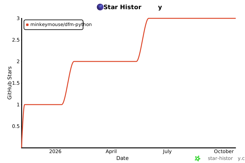
Star history
1 maintainer

Metadata
1 maintainer
Release files for dfm-python 0.8.1
For a detailed explanation of source distributions (sdists) and built distributions (wheels), please see the package formats documentation.
Source distribution (sdist)
| File | Size | Uploaded | Provenance | |
|---|---|---|---|---|
| dfm_python-0.8.1.tar.gz | 3.4 MB | With provenance | Details |
Built distribution (wheel)
| File | Interpreter | ABI | Platform | Reset |
|---|---|---|---|---|
| dfm_python-0.8.1-py3-none-any.whl | Python 3 | none | any | Details |
Total release size: 3.8 MB
Release files / dfm_python-0.8.1.tar.gz
| Download URL | dfm_python-0.8.1.tar.gz |
|---|---|
| Size | 3.4 MB |
| Tags | Source |
|
SHA-256 checksum How to use checksums |
390a48c4fb8359897d5bc4af73f281e52ecd78cd9cb12b8150215aad0cf4fadb
|
|
BLAKE2b-256 checksum How to use checksums |
395d3ee0b0e6b40492053636949ce307b803b1122bc3a6ac5864758921d808ae
|
| Upload date | |
|
Uploaded using Trusted Publishing? What is trusted publishing? |
Yes |
| Uploaded via |
twine/7.0.0 CPython/3.13.14
|
Provenance
Provenance describes where a file came from. On PyPI, provenance is shared via attestations, which provide a verifiable record of the build or publishing details. View details, limitations and caveats.


PyPI Publish Attestation
PyPI verified that this artifact, at this checksum, originated from the publisher listed below.
Signed by GitHub Actions, verified by PyPI on Oct 20, 2026.
Transparency logRelease files / dfm_python-0.8.1-py3-none-any.whl
| Download URL | dfm_python-0.8.1-py3-none-any.whl |
|---|---|
| Size | 390.8 kB |
| Tags | Python 3 |
|
SHA-256 checksum How to use checksums |
9ab58d0906cea4db1e620dd3116cbea1cd6c638732eafaf353227ea3b7a54d6a
|
|
BLAKE2b-256 checksum How to use checksums |
8f62d9e925e910ef230fe961d36c98178f404be71dbffe94109c3107a0bdb339
|
| Upload date | |
|
Uploaded using Trusted Publishing? What is trusted publishing? |
Yes |
| Uploaded via |
twine/7.0.0 CPython/3.13.14
|
Provenance
Provenance describes where a file came from. On PyPI, provenance is shared via attestations, which provide a verifiable record of the build or publishing details. View details, limitations and caveats.
PyPI Publish Attestation
PyPI verified that this artifact, at this checksum, originated from the publisher listed below.
Signed by GitHub Actions, verified by PyPI on Oct 20, 2026.
Transparency logSecurity for dfm-python 0.8.1
Provenance
Provenance describes where a file came from. On PyPI, provenance is shared via attestations, which provide a verifiable record of the build or publishing details. View details, limitations and caveats.
Full provenance
All 2 files in this release have been uploaded with provenance metadata.
Attestation for dfm_python-0.8.1.tar.gz
PyPI Publish Attestation
PyPI verified that this artifact, at this checksum, originated from the publisher listed below.
Signed by GitHub Actions, verified by PyPI on Oct 20, 2026.
Transparency logA note on package security
PyPI is a repository for distributing packages, not a service for auditing them. While third-party security researchers and our staff do their best to detect and remove malicious packages, PyPI cannot guarantee the quality, security or suitability of any given package.














