
D'Hondt-projected removal-effect attributions for tabular XAI

Project description
DhondtXAI
DhondtXAI is a D'Hondt-based post-hoc attribution library for tabular models. It explains row-wise numeric model scores with removal effects, signed evidence votes, proportional D'Hondt allocation, and completeness-preserving projection.
DhondtXAI can explain any tabular model that can be adapted to a row-wise numeric scoring function. It includes automatic adapters for common model families such as sklearn-style estimators, XGBoost, LightGBM, CatBoost, PyTorch modules, and Keras-like models.
Status: DhondtXAI 0.9.5.5 is an experimental/beta tabular XAI library. It is suitable for research, model inspection, and controlled pilot use. For high-stakes deployment, validate explanations against task-specific benchmarks and compare them with established methods such as SHAP and LIME.
Install
pip install dhondtxai==0.9.5.5
For local development from this repository:
pip install -e .[dev]
scikit-learn and other ML frameworks are optional for the core library. Use
extras when you want adapter dependencies:
pip install "dhondtxai[sklearn]"
pip install "dhondtxai[xgboost]"
pip install "dhondtxai[lightgbm]"
pip install "dhondtxai[catboost]"
pip install "dhondtxai[torch]"
pip install "dhondtxai[all-models]"
Quick Start
The shortest path is the one-call API:
import dhondtxai as dxai

explanation = dxai.explain(
    model,
    X_background=X_train,
    X=X_test.iloc[0],
    task="classification",
    output="probability",
    target="predicted",
)

print(explanation.values)
print(explanation.report())
explanation.plot(kind="waterfall")
For repeated explanations, create an explainer once:
import pandas as pd
from sklearn.datasets import load_breast_cancer
from sklearn.ensemble import RandomForestClassifier
from sklearn.model_selection import train_test_split

from dhondtxai import Explainer

dataset = load_breast_cancer()
X = pd.DataFrame(dataset.data, columns=dataset.feature_names)
y = pd.Series(dataset.target)

X_train, X_test, y_train, y_test = train_test_split(
    X, y, test_size=0.3, random_state=42, stratify=y
)

model = RandomForestClassifier(n_estimators=200, random_state=42)
model.fit(X_train, y_train)
explainer = Explainer(
    model,
    X_train,
    task="classification",
    output="probability",
    target="predicted",
    cost_mode="auto",
)

dhondtxai_values = explainer(
    X_test.head(5),
    threshold=0.05,
    redistribute=True,
)

print(dhondtxai_values.values)
print(dhondtxai_values.base_values)
print(dhondtxai_values.to_frame(row=0, top_k=10))
print(dhondtxai_values.summary(row=0))

explainer.plot_waterfall(dhondtxai_values[0], top_k=10)
dhondtxai_values.values contains additive DhondtXAI attribution arrays.
The values are not Shapley values; they are D'Hondt-projected removal-effect
attributions.
Runtime Cost Modes
DhondtXAI can trade off speed and explanation detail without changing the model prediction or the core attribution definition.
explainer = dxai.Explainer(model, X_train, cost_mode="auto")
exp = explainer.explain(X_test.iloc[0])
Available modes:
| Mode | Best for | What it does |
|---|---|---|
fast |
large data and quick debugging | fewer background rows, screened interaction pairs, lower allocation resolution |
balanced |
default analysis | moderate background and interaction screening |
accurate |
reports and deeper inspection | more background rows and more interaction pairs |
research |
benchmarks | exhaustive settings where practical |
auto |
hands-off use | chooses a policy from estimated explanation cost |
Explicit parameters such as n_background, allocation_seats,
max_interaction_pairs, and top_k_interaction_features override the selected
cost mode. Each explanation reports the resolved policy in
explanation.diagnostics()["cost"].
Runtime caps are explicit. If you pass max_model_rows, DhondtXAI screens
interaction pairs and caps background rows so the estimated perturbation rows
stay within the budget, or raises a clear error when the budget is impossible.
allocation_error_tolerance is a convenience way to choose D'Hondt allocation
resolution from an approximate score scale. It is not a formal per-feature
error guarantee; D'Hondt remains a highest-averages allocation rule.
For custom or unusual models, provide a row-wise numeric scoring function:
explainer = Explainer.from_score_function(
    score_fn=my_score_function,
    background_data=X_train,
    feature_names=X_train.columns,
)
The practical compatibility rule is simple: DhondtXAI supports tabular models that can be converted into a row-wise numeric scoring function.
Maskers provide a compact way to describe how hidden features are replaced:
masker = dxai.maskers.Independent(X_train)
explainer = dxai.Explainer(model, masker=masker, output="probability")
Available lightweight maskers are Independent, ConditionalKNN, and
UserDefined. They map to DhondtXAI's existing tabular perturbation modes.
When a masker has max_samples, that value becomes the default background
sample count unless explain(n_background=...) is explicitly provided.
Baseline Mode
DhondtXAI reports the model difference relative to a baseline. By default the baseline is computed over the full background dataset:
exp = explainer.explain(x, baseline_mode="full")
Removal effects may use a sampled background for runtime. If you want the baseline and removal effects to use the same sampled rows, use:
exp = explainer.explain(x, baseline_mode="sample")
This can reduce projection correction for additive models when
n_background is small. Diagnostics include full_baseline,
sample_baseline, baseline_sampling_gap, and the active baseline_mode.
Attribution Values API
The recommended public API uses a familiar explainer workflow:
import dhondtxai as dxai

explainer = dxai.Explainer(model, X_background)
dhondtxai_values = explainer(X_to_explain)

dhondtxai_values.values          # numpy attribution array
dhondtxai_values.dhondtxai_values # alias for values
dhondtxai_values.base_values     # baselines
dhondtxai_values.scores          # model scores explained by DhondtXAI
dhondtxai_values.feature_names   # feature order
For a single row, dhondtxai_values.values has shape (n_features,). For a
table, it has shape (n_rows, n_features). Detailed local objects are still
available:
local_explanation = dhondtxai_values[0]
local_explanation.dhondtxai_values
local_explanation.to_feature_frame()
local_explanation.summary()
Residual categories such as excluded or below-threshold effects are stored in
dhondtxai_values.residual_values so the main value matrix remains aligned with
the original feature columns.
Plots render residuals with friendly labels by default. For example,
__projection_residual__ is shown as
projection correction (not a feature) so it is not mistaken for a model input.
Use residuals="show", "hide", or "separate" in local plots.
Single-row explanations also keep the same column order:
local_explanation.feature_names
local_explanation.values
Both arrays follow the original background/model feature order, not the order of manual alliance members.
DhondtXAI validates the explanation path aggressively: duplicate feature names, non-finite model scores, and negative/non-finite D'Hondt votes fail with clear errors instead of producing silent attributions.
Three Core User Controls
Most DhondtXAI use cases can be configured with three user-facing controls:
user_alliances: manually group related variables by their column names.threshold: set the explanatory vote barrier.seats: set the visible parliament size.
import dhondtxai as dxai
from dhondtxai import plot_signed_parliament

explainer = dxai.Explainer(model, X_train)

explanation = explainer.explain(
    X_test.iloc[0],
    alliance_mode="user",
    user_alliances=[
        ["mean radius", "mean perimeter", "mean area"],
        ["mean concavity", "mean concave points"],
        ["worst radius", "worst perimeter", "worst area"],
    ],
    threshold=0.05,       # 5 percent barrier
    redistribute=True,    # transfer below-threshold votes to related alliances
    seats=200,            # visible parliament size
    n_background=50,
)

print(explanation.to_feature_frame(top_k=10))
print(explanation.to_alliance_frame())

plot_signed_parliament(
    explanation,
    mode="signed",
    seat_count=200,
)
Manual alliances use the exact column names from the background DataFrame.
If a name is misspelled, DhondtXAI raises an error by default
(strict_features=True) instead of silently ignoring it.
Set alliance_mode="none" when every variable should stand alone. Use
alliance_mode="auto" when DhondtXAI should infer alliances from interaction
affinity. Use alliance_mode="hybrid" when you want to provide some manual
alliances and let the remaining variables be grouped automatically.
Threshold behavior is explicit:
threshold=Noneorthreshold_enabled=False: no barrier.threshold=0.05: alliances need at least 5 percent of explanatory vote.redistribute=True: below-threshold votes are transferred by affinity.redistribute=False: below-threshold contribution is reported separately as__below_threshold__.threshold_mode="strict_residual"is the default. If a below-threshold feature interacts with an eligible feature, the interaction is kept in the below-threshold residual instead of being silently assigned to the eligible feature.
Seat behavior is separated from numerical attribution:
seats: visible parliament size, for example 100, 200, or 300.allocation_seats: high-resolution internal D'Hondt allocation used for the continuous DhondtXAI values.- if
allocation_seatsis omitted, DhondtXAI chooses a high-resolution default.
Two additional reliability controls are available when needed:
exclude_mode="strict"is the default and keeps excluded-feature interaction effects in__excluded__.projection_mode="auto"is the default and creates a__projection_residual__row when raw D'Hondt evidence is absent or when the projection correction is large relative to the raw evidence. The defaultprojection_residual_threshold=0.10keeps corrections of 10 percent or more separate. Useprojection_mode="redistribute"only when you intentionally want every projection correction distributed to features.
Method Summary
For a trained model score g_c(x), DhondtXAI computes a baseline
mu_c = E[g_c(X)]
and the local model difference
Delta_c(x) = g_c(x) - mu_c
For a feature or feature alliance A, the method estimates a
background-interventional removal score
R_A^D(x) = (1 / M) sum_m g_c(x_-A, z_A^(m))
and the local removal effect
e_A^D(x) = g_c(x) - R_A^D(x)
The samples z_A^(m) come from the background data provided through fit(...)
or background_data. This is not a Shapley-value or SHAP computation.
These effects are converted into positive and negative explanatory votes. The D'Hondt rule allocates explanatory seats separately for supporting and opposing evidence. Signed source back-projection keeps positive and negative source effects separate. A final conservative projection, or an explicit projection residual bucket, maps the representation back onto the model difference:
sum_i phi_i^D(x) = g_c(x) - mu_c
DhondtXAI therefore produces signed additive local attributions, but the values should be interpreted as D'Hondt-projected removal-effect attributions rather than Shapley values.
Main Features
- D'Hondt-projected local feature attributions.
- Background-interventional feature removal using a background dataset.
- Optional conditional KNN perturbation for more local replacements.
- Manual, automatic, hybrid, or no feature alliances.
- Same-direction or absolute-interaction affinity for automatic alliances.
- Optional threshold/barrier mechanism.
- Optional redistribution of below-threshold alliance votes.
- Positive and negative D'Hondt evidence parliaments.
- Explicit stable or random D'Hondt tie-breaking.
- Excluded-feature and below-threshold residual reporting.
- Projection residual diagnostics.
- Separate attribution resolution and display seat counts.
- Local and global explanation outputs.
- Global alliance co-occurrence matrix for automatic/hybrid alliances.
- Backward-compatible legacy
feature_importances_allocation API.
Comparison With Existing XAI Methods
DhondtXAI does not compute SHAP values or approximate Shapley values. It does not average marginal contributions over all feature coalitions, and its explanations should not be interpreted as Shapley values. It is a separate D'Hondt-based attribution operator that can be compared with SHAP, LIME, or permutation-based explanations in experiments.
When To Use
Use DhondtXAI when you want signed local feature attributions, alliance-level explanations, threshold/barrier analysis, parliamentary representation of model evidence, and global alliance co-occurrence analysis.
Local Explanation Example
import pandas as pd
from sklearn.datasets import load_breast_cancer
from sklearn.ensemble import RandomForestClassifier
from sklearn.model_selection import train_test_split

from dhondtxai import Explainer, plot_signed_parliament

dataset = load_breast_cancer()
X = pd.DataFrame(dataset.data, columns=dataset.feature_names)
y = pd.Series(dataset.target)

X_train, X_test, y_train, y_test = train_test_split(
    X,
    y,
    test_size=0.3,
    random_state=42,
    stratify=y,
)

model = RandomForestClassifier(n_estimators=200, random_state=42)
model.fit(X_train, y_train)
explainer = Explainer(model, X_train)

explanation = explainer.explain(
    X_test.iloc[0],
    seats=120,
    allocation_seats=5000,
    threshold=0.05,
    redistribute=True,
    alliance_mode="user",
    user_alliances=[
        ["mean concavity", "mean concave points"],
        ["mean radius", "mean perimeter", "mean area"],
    ],
    n_background=50,
    lambda_interaction=0.2,
)

print(explanation.to_feature_frame())
print(explanation.to_alliance_frame())
print(explanation.summary(top_k=5))
print(explanation.diagnostics())
print(explanation.projection_residual_ratio)

explainer.plot_local_bar(explanation, top_k=10)
explainer.plot_waterfall(explanation, top_k=10)
plot_signed_parliament(explanation, mode="signed")
Model Compatibility
DhondtXAI can explain any tabular model that maps input rows to numeric scores. It does not require model internals, gradients, tree structure, or SHAP values.
Supported model families:
- sklearn estimators and sklearn
Pipelineobjects - XGBoost sklearn estimators
- native XGBoost
Booster - native LightGBM
Booster - CatBoost estimators
- PyTorch
nn.Module - Keras-like models
- custom scoring functions
The recommended API does not require you to call model-specific scoring methods
yourself. The default model_adapter="auto" and input_format="auto" select an
input format automatically:
| Model family | Typical object | Automatic input |
|---|---|---|
| sklearn / sklearn Pipeline | RandomForestClassifier, Pipeline, XGBClassifier sklearn API |
pandas DataFrame |
| native XGBoost | xgboost.Booster |
xgboost.DMatrix |
| native LightGBM | lightgbm.Booster |
pandas DataFrame |
| CatBoost | CatBoostClassifier, CatBoostRegressor |
pandas DataFrame |
| PyTorch | torch.nn.Module |
torch.float32 tensor |
| Keras-like | Keras-compatible model object | NumPy array |
| custom | row-wise scoring function | controlled by input_format or input_adapter |
For already-trained models, you can pass the background data directly:
explainer = Explainer(trained_model, X_train)
dhondtxai_values = explainer(X_test)
For unusual models, remote services, ONNX wrappers, sparse inputs, or models with custom output formats, wrap them into a row-wise numeric score:
explainer = Explainer(
    score_fn=lambda X: my_service_score(X),
    background_data=X_train,
)
You can also pass framework-specific prediction keyword arguments and an output adapter:
explainer = Explainer(
    booster,
    X_train,
    output="prediction",
    predict_kwargs={"raw_score": True},
    output_adapter=lambda raw: raw[:, 1] if raw.ndim == 2 else raw,
)
output="logit" means probability log-odds computed from the selected
probability. For native raw margins/logits, use output="prediction" with
predict_kwargs or a score_fn.
When output="probability" is selected, DhondtXAI validates that the selected
scores are finite probabilities in [0, 1]. If your model returns logits or raw
margins, apply sigmoid/softmax with output_adapter, or choose
output="prediction" / output="decision" instead.
XGBoost
sklearn-style XGBoost estimators work directly:
from xgboost import XGBClassifier

model = XGBClassifier(...).fit(X_train, y_train)

explainer = Explainer(model, X_train)
dhondtxai_values = explainer(X_test)
Native XGBoost Booster objects are adapted automatically:
import xgboost as xgb

dtrain = xgb.DMatrix(X_train, label=y_train, feature_names=list(X_train.columns))
booster = xgb.train({"objective": "binary:logistic"}, dtrain)

explainer = Explainer(booster, X_train)
dhondtxai_values = explainer(X_test)
For native binary boosters, DhondtXAI uses the numeric score returned by the booster as the explained model output.
LightGBM
import lightgbm as lgb

dataset = lgb.Dataset(X_train, label=y_train)
booster = lgb.train({"objective": "binary"}, dataset)

explainer = Explainer(booster, X_train)
dhondtxai_values = explainer(X_test)
CatBoost
from catboost import CatBoostClassifier

model = CatBoostClassifier(verbose=False).fit(X_train, y_train)

explainer = Explainer(model, X_train)
dhondtxai_values = explainer(X_test)
PyTorch
import torch

class Net(torch.nn.Module):
    def forward(self, X):
        return torch.sigmoid(self.linear(X)).squeeze(-1)

model = Net()

explainer = Explainer(model, X_train)
dhondtxai_values = explainer(X_test)
DhondtXAI converts tabular rows to torch.float32 tensors automatically.
If your neural model returns logits, convert them explicitly:
explainer = Explainer(
    torch_model,
    X_train,
    task="classification",
    output="probability",
    output_adapter=lambda y: torch.softmax(torch.as_tensor(y), dim=1).detach().cpu().numpy(),
)
Keras-like Models
explainer = Explainer(
    keras_model,
    X_train,
    model_adapter="keras",
)

dhondtxai_values = explainer(X_test)
Keras-like models receive NumPy arrays by default.
Binary neural models that return a one-dimensional sigmoid probability or a
single-column (n, 1) probability matrix are handled as binary probabilities:
class 1 uses p, class 0 uses 1 - p.
For custom, Keras, PyTorch, ONNX, or remote models, pass a callable:
def score_fn(X):
    return my_model_score_function(X)

explainer = Explainer(
    score_fn=score_fn,
    background_data=X_train,
)
If your model expects NumPy arrays instead of pandas DataFrames:
explainer = Explainer(
    score_fn=lambda X: keras_model.predict(X, verbose=0)[:, 1],
    background_data=X_train,
    input_format="numpy",
)
For more complex conversions, use input_adapter:
explainer = Explainer(
    score_fn=score_fn,
    background_data=X_train,
    input_adapter=lambda X: X.to_numpy(dtype="float32"),
)
When automatic inference is not enough, override the adapter explicitly:
explainer = Explainer(
    model,
    X_train,
    model_adapter="xgboost",   # sklearn, xgboost, lightgbm, catboost, torch, keras
    input_format="auto",
)
For multi-output regression or custom score matrices, select the target column:
explainer = Explainer(
    model,
    X_train,
    target_index=1,
)
For convenience, target=1 is also treated as target_index=1 when the
resolved output type is prediction or custom. For classifiers, prefer
target="predicted", a class label, or an explicit class_index.
For custom two-dimensional score matrices, target_index has priority. If it
is not provided, class_index is used, including class_index="predicted" for
argmax-based local class selection.
For multiclass classification, you may explain the predicted class directly:
explanation = explainer.explain(
    X_test.iloc[0],
    class_index="predicted",
)
Check compatibility before running a large explanation job:
print(explainer.check_model_compatibility())
If no background data has been set yet, pass a sample directly:
print(explainer.check_model_compatibility(X_sample=X_train.head()))
Alliance Modes
alliance_mode="none" treats each feature as its own actor.
alliance_mode="user" uses only user-defined disjoint alliances and keeps
remaining features as individual actors.
alliance_mode="auto" estimates pairwise interaction affinity and forms
automatic alliances. Use auto_alliance_method="connected_components" for the
default graph component rule or auto_alliance_method="complete_linkage" for a
stricter rule requiring all pairs inside an alliance to meet the affinity
threshold.
alliance_mode="hybrid" preserves user-defined alliances and applies automatic
alliance formation only to the remaining features.
Threshold And Redistribution
Set threshold=None or threshold_enabled=False to disable the barrier system.
Set threshold=0.05 to require at least 5 percent of the explanatory vote.
If redistribute=True, below-threshold alliance votes are transferred to
eligible alliances according to affinity. If redistribute=False, below-threshold
alliances are reported but do not receive seats. Their model contribution is
kept in __below_threshold__ and explanation.below_threshold_residual instead
of being forced into eligible features.
The default threshold_mode="strict_residual" also keeps interactions involving
below-threshold features in the below-threshold residual. Use
threshold_mode="standard" for the older removal-effect semantics.
If exclude_features=[...] is used, excluded feature influence is not assigned
to the remaining active features. It is reported through __excluded__ and
explanation.excluded_residual.
By default this uses exclude_mode="strict". In interaction-heavy models, this
means interactions involving excluded variables are also kept in the excluded
residual. exclude_mode="standard" is available for legacy behavior where
active-feature effects are computed while excluded features stay fixed at their
explained-row values.
Attribution Resolution And Display Seats
allocation_seats controls the numerical D'Hondt resolution used to compute
continuous attributions. Larger values reduce integer seat rounding effects.
seats controls the visible parliament size used in the plotted explanation.
For example, allocation_seats=10000 and seats=100 produces a high-resolution
attribution with a compact 100-seat visualization.
If allocation_seats is not provided, DhondtXAI uses:
max(5000, 100 * number_of_active_features, seats)
This default prevents small display parliaments such as seats=10 from
zeroing out meaningful low-rank features in the numerical attribution.
Perturbation, Affinity, And Tie-Breaking
perturbation="interventional" is the default. It replaces the removed feature
or feature group with values sampled from the background data:
g_c(x_-A, z_A)
perturbation="conditional_knn" uses nearest background rows according to the
non-removed features before taking replacement values. This is still an
approximation, but it reduces unrealistic replacements when correlated tabular
features are present.
For domain-specific replacements, use perturbation="user_sampler":
def sampler(x, group, background, n):
    rows = background.sample(n=n, replace=True, random_state=42).reset_index(drop=True)
    # edit rows[group] here using domain-specific rules
    return rows

explainer = Explainer(
    model,
    X_train,
    perturbation="user_sampler",
    perturbation_sampler=sampler,
)
Automatic alliances can use:
affinity_mode="same_direction": only same-sign single-feature effects can form high-affinity alliances.affinity_mode="absolute_interaction": pairwise interaction magnitude can create affinity even when single-feature effects are weak or opposite.
D'Hondt ties are explicit:
tie_break="stable": deterministic order-preserving tie-break.tie_break="random": seeded random tie-break usingrandom_state.
Stable tie-breaking is reproducible but can favor earlier feature/alliance
order in exact ties. Increase allocation_seats to reduce the practical impact
of integer ties.
D'Hondt votes must be finite and non-negative. Negative model evidence is handled through separate positive/negative explanatory vote channels, not by passing negative election votes into the D'Hondt allocator.
Outputs
explanation.to_feature_frame() returns local feature attributions:
featureattributionabs_attributionsource_allianceeffectdirectionrelative_sharesign_consistentis_residual- residual rows such as
__excluded__or__below_threshold__when relevant __projection_residual__when projection correction is intentionally kept out of feature values
explanation.to_alliance_frame() returns alliance-level votes and seats:
votespositive_votesnegative_votespositive_seatsnegative_seatssource_attributionrepresented_attributionsource_raw_attributionrepresented_raw_attribution- threshold status
Diagnostic fields on the explanation object include:
raw_attribution_sumprojection_targetprojection_residualprojection_residual_ratioprojection_residual_attributionexcluded_residualbelow_threshold_residualresolved_output_typeperturbationaffinity_modetie_breakprojection_modeexclude_modethreshold_mode
Global Explanation
explanations = explainer.explain_many(
    X_test.head(50),
    random_state=42,
    reuse_background_sample=False,
    n_background=50,
)

global_frame = explainer.explain_global(
    X_test,
    max_rows=50,
    random_state=42,
    reuse_background_sample=False,
    seats=100,
    alliance_mode="none",
    n_background=50,
)

print(global_frame)
print(explainer.global_alliance_matrix_)

explainer.plot_global_importance(global_frame)
explainer.plot_global_alliance_heatmap()
The global output includes:
global_abs: mean absolute DhondtXAI attributiondirectional: mean signed attributionpositive: mean positive attributionnegative: mean negative attributionthreshold_survival: frequency of threshold eligibilityis_residual: marks__excluded__,__below_threshold__, and__projection_residual__rows
By default, global explanations use controlled but different background samples
for each row. Set reuse_background_sample=True when you want the same random
background sample reused across all rows.
Diagnostics And Reports
print(explanation.summary(top_k=8))
print(explanation.diagnostics())
Public reports and plot labels are English-only. Passing any value other than
language="en" raises a clear error.
projection_residual_ratio should be monitored. A low value means the raw
D'Hondt representation naturally matches the local model difference; a high
value means the conservative projection made a larger correction and the
explanation should be interpreted with more caution.
Interpretation guide:
0.00 - 0.10: low correction; explanation is closer to raw D'Hondt evidence.0.10 - 0.50: medium correction; interpret with caution.> 0.50: high correction; raw D'Hondt evidence required a large projection.
The text report and plots print an explicit warning when this correction is
medium or high. If __projection_residual__ appears in the output, the raw
D'Hondt evidence did not support assigning that correction to individual
features under the selected projection_mode.
diagnostics()["mixed_sign_alliance_count"] reports alliances that contain both
supporting and opposing member-level effects. When this count is non-zero,
interpret parliament seats together with explanation.to_feature_frame().
Plots
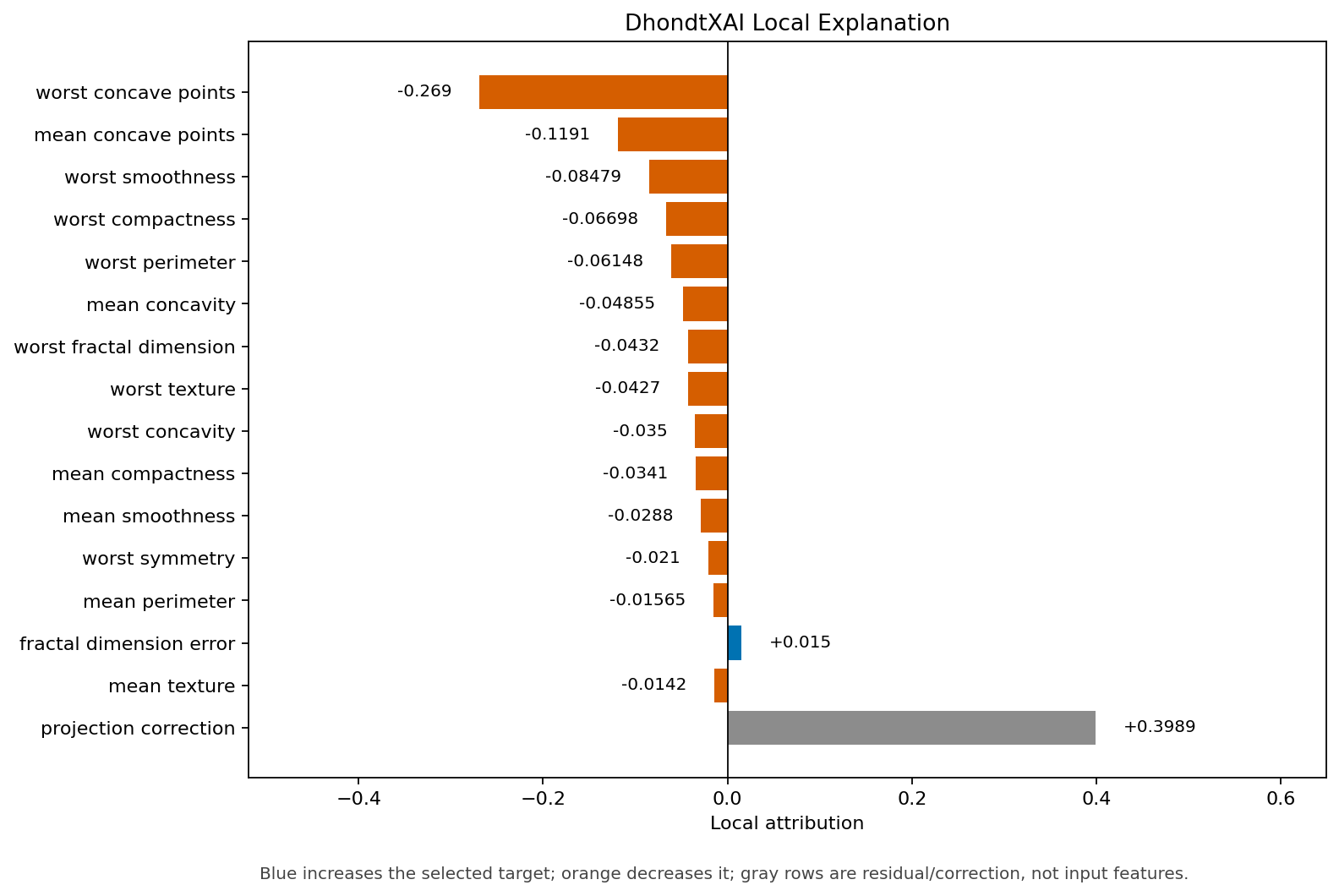
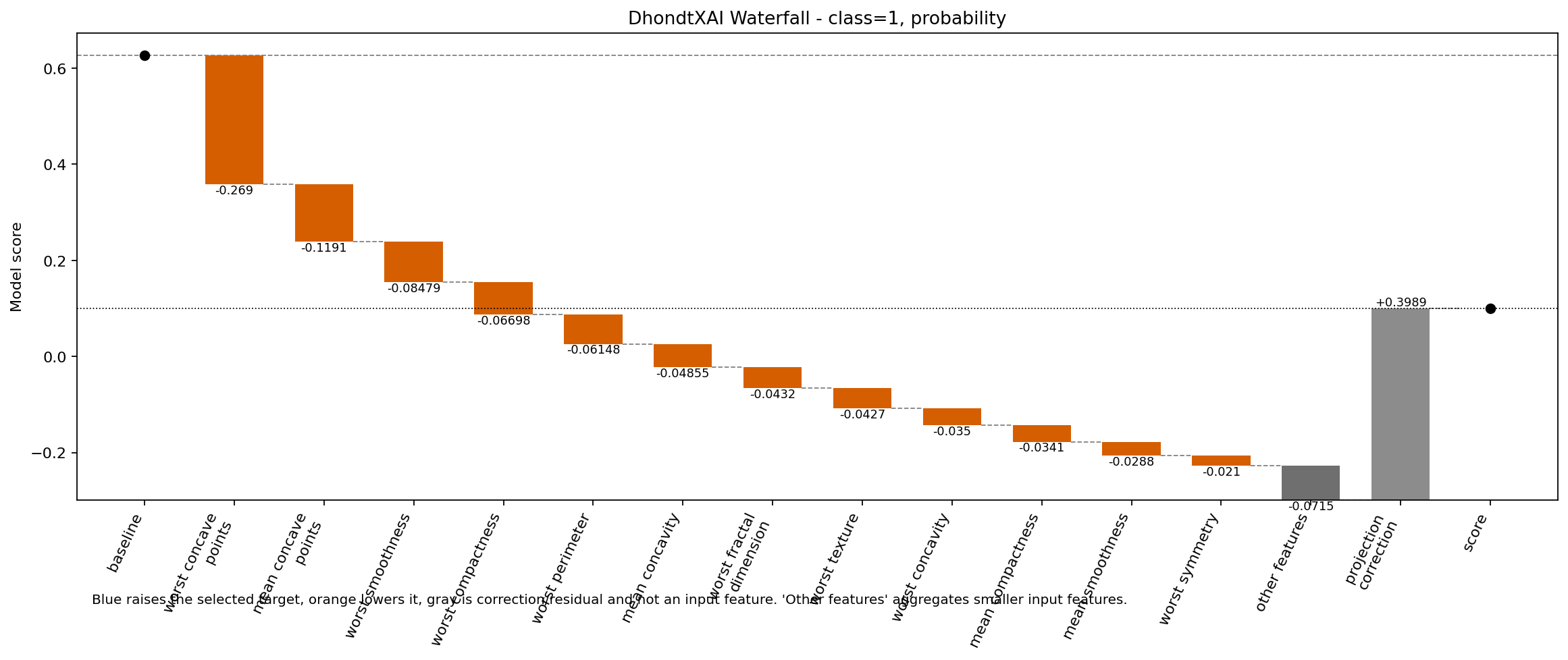
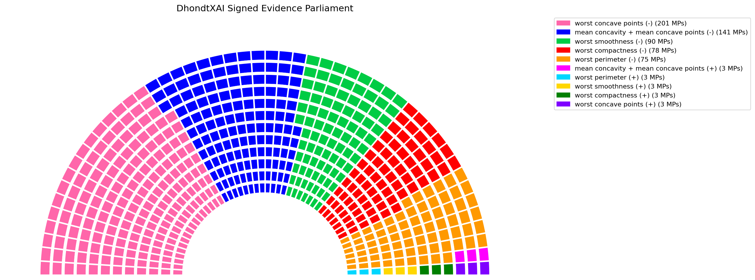
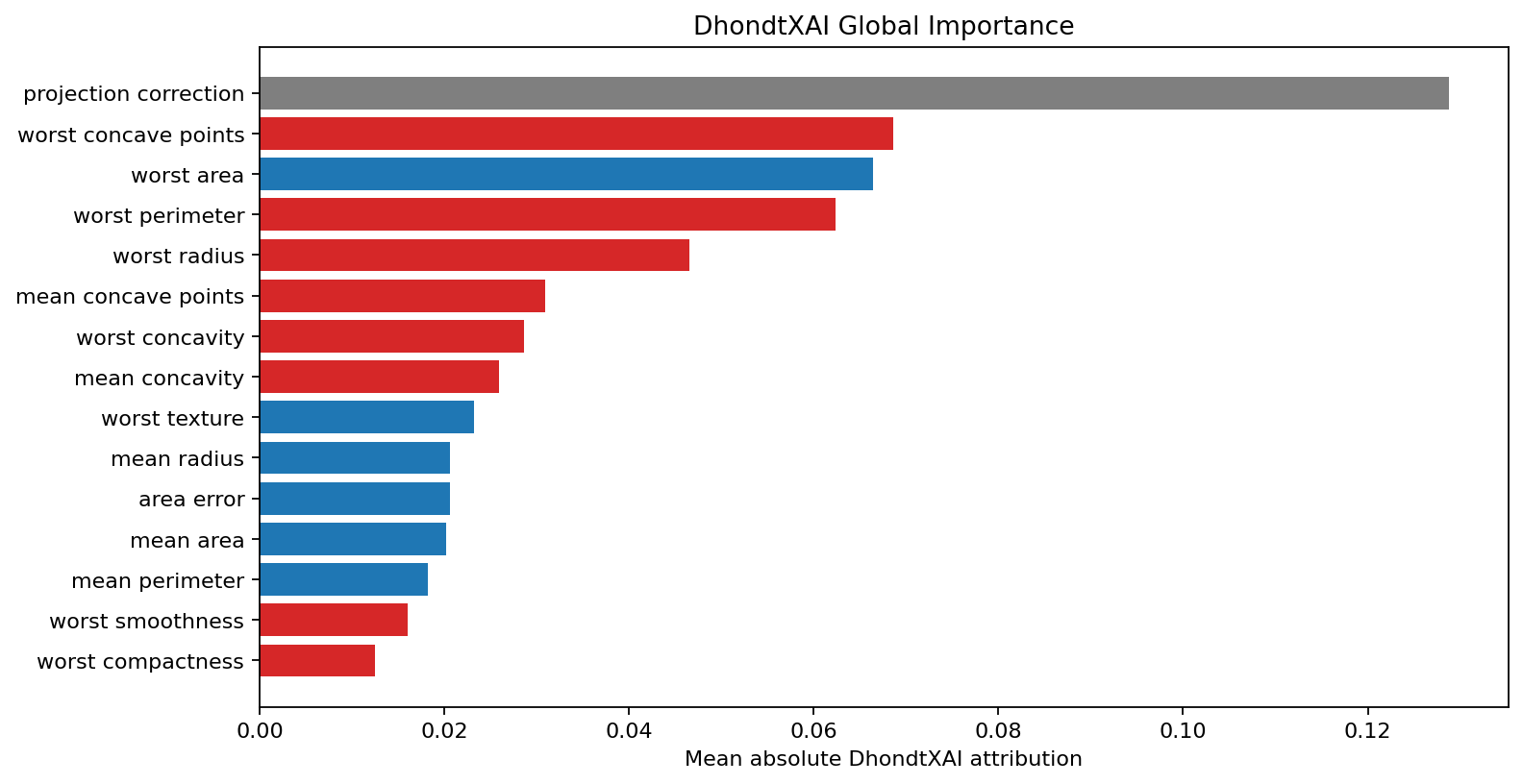
plot_local_bar(...): signed local feature bar plot.plot_waterfall(...): baseline-to-score additive waterfall.plot_signed_parliament(...): positive/negative evidence parliament.plot_global_importance(...): residual-aware global importance.plot_global_alliance_heatmap(...): global alliance co-occurrence matrix.
Parliament plots are a core DhondtXAI output. The user controls the requested
seat count through seats in explain(...) or seat_count in
plot_signed_parliament(...). The visual layer uses a high-contrast qualitative
palette by default: positive evidence uses blue/green/cyan tones and negative
evidence uses orange/red/pink tones. This keeps direction visually clear while
still giving different alliances separable colors. Use palette="distinct" if
you prefer a fully qualitative palette independent of sign.
For readability, awkward display totals are snapped to clean counts by default:
multiples of 10 for small parliaments, 50 for medium parliaments, and 100 for
larger parliaments. For example, a 257-seat request is visualized as 250 seats
unless snap_seats=False is passed. This affects only the display; numerical
attributions use allocation_seats.
The parliament geometry uses a smaller inner half-circle so the evidence ring is visually denser and closer to the legacy DhondtXAI parliament view.
explanation = explainer.explain(X_test.iloc[0], seats=257)

plot_signed_parliament(
    explanation,
    mode="signed",
    seat_count=257,
    palette="signed",
    snap_seats=True,
)
Example visual outputs are included in exampleimages/:
Waterfall plots separate residual/correction rows from real features. When
top_k hides smaller input features, they are grouped as other features,
which is an aggregate of input features rather than a correction term.
Regenerate them with:
MPLBACKEND=Agg python examples/generate_visual_examples.py
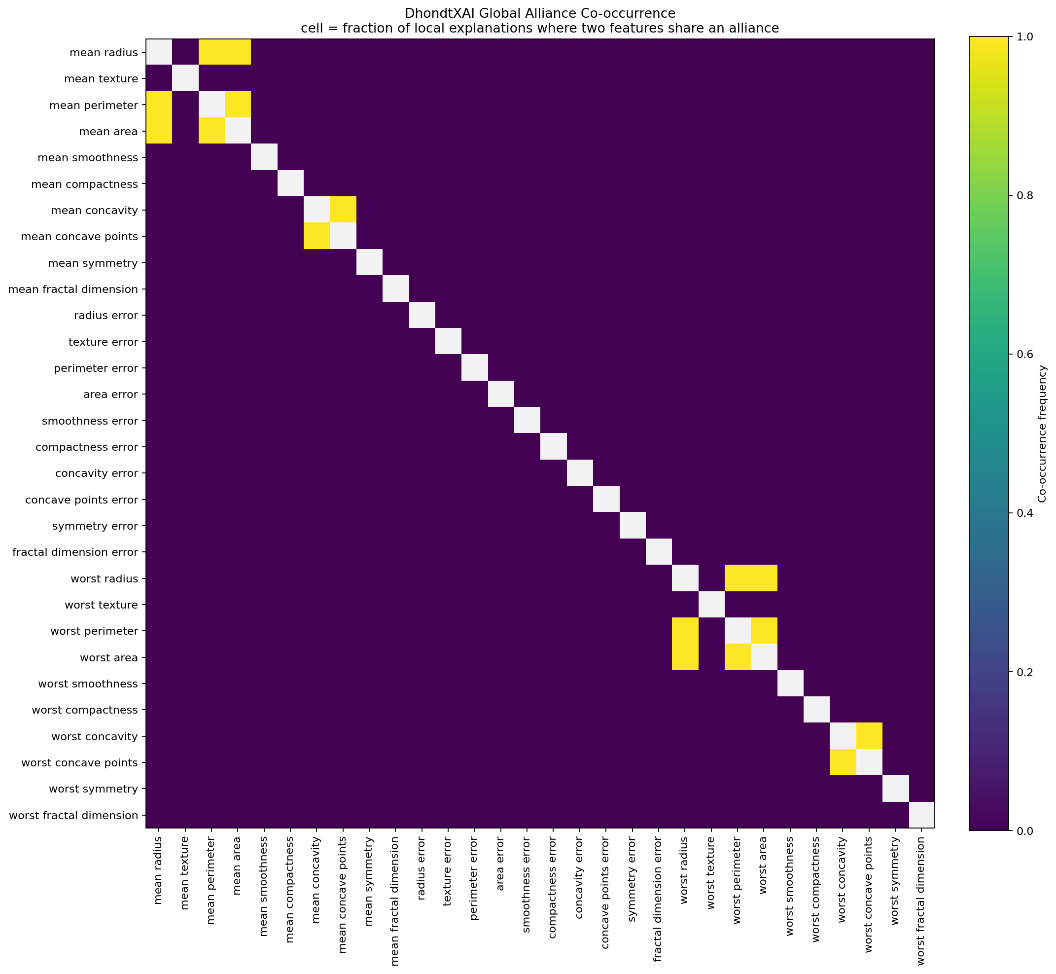
The global alliance heatmap is not a generic correlation plot. Each cell is the
fraction of local explanations in which two features appear in the same
DhondtXAI alliance. If every feature is explained as a singleton
(alliance_mode="none"), the off-diagonal matrix is empty by design and the
plot reports that no repeated feature co-occurrence was found. Use
alliance_mode="auto", alliance_mode="hybrid", or user_alliances when you
want this matrix to carry alliance-structure information.
Limitations
- DhondtXAI is a beta tabular XAI library, not a mature SHAP/LIME replacement.
- Current removal sampling is background-interventional, not fully conditional.
conditional_knnis an approximate local sampler, not a causal conditional distribution estimator.user_samplercan improve domain realism, but its validity depends on the sampler supplied by the user.- Low
allocation_seatsvalues can produce sparse or order-sensitive attributions; the default uses high-resolution allocation. - Stable D'Hondt tie-breaking is order-preserving and should be documented when exact ties matter.
- D'Hondt input votes must be finite and non-negative; signed evidence is represented through separate positive and negative channels.
- Background replacement can create out-of-distribution rows for strongly correlated features.
- Auto-alliance and interaction estimation can be expensive for high-dimensional data.
- Projection residuals should be monitored and reported.
projection_mode="auto"keeps zero-evidence and high-correction projections in__projection_residual__; useprojection_mode="redistribute"only when you intentionally want every projection correction distributed to features.- Probability-scale explanations may be less additive than logit-scale explanations.
- Below-threshold and excluded residuals should be interpreted explicitly.
Building A PyPI-Ready Package
The package metadata includes README long description, version, license, citation, and optional sklearn/dev extras. To build local distribution files:
python -m pip install --upgrade build twine
python -m build
python -m twine check dist/*
Then a built wheel can be installed locally with:
pip install dist/dhondtxai-0.9.5.5-py3-none-any.whl
Publishing to PyPI requires a PyPI API token:
python -m twine upload dist/*
Legacy API
The previous global feature-importance workflow is still available:
features, votes, excluded = explainer.apply_dhondt(
    num_votes=100000000,
    num_mps=600,
    threshold=5,
)

seats = explainer.dhondt_method(votes, 600, excluded)
explainer.plot_results(features, seats)
This legacy path uses model.feature_importances_. The new proposed method is
explain(...).
Citation
T. B. Donmez, "Explainable AI through a Democratic Lens: DhondtXAI for Proportional Feature Importance Using the D'Hondt Method," 2024. https://doi.org/10.48550/arXiv.2411.05196
Release history Release notifications | RSS feed


Download files
Download the file for your platform. If you're not sure which to choose, learn more about installing packages.
Source Distribution
Built Distribution
Filter files by name, interpreter, ABI, and platform.
If you're not sure about the file name format, learn more about wheel file names.
Copy a direct link to the current filters
File details
Details for the file dhondtxai-0.9.5.5.tar.gz.
File metadata
- Download URL: dhondtxai-0.9.5.5.tar.gz
- Upload date:
- Size: 2.1 MB
- Tags: Source
- Uploaded using Trusted Publishing? No
- Uploaded via: twine/6.2.0 CPython/3.12.12
File hashes
| Algorithm | Hash digest | |
|---|---|---|
| SHA256 |
9d354c7a6dda254c25fe16ebcbea67ae1b626d05afd1eda54c0b578040fc5c39
|
|
| MD5 |
e44f917b68ea8fc0ed5cfe5bc52297b9
|
|
| BLAKE2b-256 |
be86e63cb0cd49d455620bc0788835d75cfa8b08f7c5766e2fd41a85a8fc28b9
|
File details
Details for the file dhondtxai-0.9.5.5-py3-none-any.whl.
File metadata
- Download URL: dhondtxai-0.9.5.5-py3-none-any.whl
- Upload date:
- Size: 49.6 kB
- Tags: Python 3
- Uploaded using Trusted Publishing? No
- Uploaded via: twine/6.2.0 CPython/3.12.12
File hashes
| Algorithm | Hash digest | |
|---|---|---|
| SHA256 |
1dfa34742ebd51e1033b6195fe7dbc1069d9712f8662044605025ed23d8d6f86
|
|
| MD5 |
44eb74d2634cbceca853ca4d7d79bd0d
|
|
| BLAKE2b-256 |
2f67e2a48cb664b63c278be2236d44192c8b41bff6f3e2a89199e02df1fc9d1a
|






