
DichromaticMap
DichromaticMap provides a Python library and an interactive viewer for layer-resolved SC/FCC/BCC tilt grain-boundary dichromatic patterns. Use it to inspect two overlaid grains, identify coincidence sites, measure crystal vectors, count atoms in selected cells and explore common cells under uniform strain.
Features
- Simple cubic (SC), face-centered cubic (FCC) and body-centered cubic (BCC) lattices with ⟨100⟩, ⟨110⟩, ⟨111⟩, ⟨112⟩ and custom integer tilt axes.
- Independent grain/layer visibility, grain-boundary side filtering, display rotation, floating grain reference axes, custom grain colors and unique layer symbols.
- Same-layer exact coincidence-site lattice (CSL) detection and local near-pair matching.
- Vector measurements in both grain coordinate frames, including axial periodic images.
- Manual common cells with separate G1/G2 atom counts and optional uniform strain fitting.
- Automatic homogeneous-strain common-cell search and PNG export.
- Save and restore sessions, with count, vector and strain CSV tables in one file.
- NumPy-based numerical functions usable independently of the viewer.
The three choices represent cubic Bravais point lattices with one atom per primitive cell. Structures with an additional multi-atom basis, such as diamond, are not represented. FCC remains the default.
Coordinates and distances use the reference lattice constant a₀ as their unit. Local matching preserves the atom positions. Strain operations impose a geometric deformation; they do not perform atomic relaxation or minimize elastic energy. A manually selected polygon alone does not establish crystal periodicity.
Install and launch
Requires Python 3.10 or later. Install the library and viewer from PyPI:
python -m pip install "dichromatic-map[gui]"
python -m dichromatic_map
The viewer uses PySide6 and PyQtGraph. For numerical calculations only, install
with python -m pip install dichromatic-map; the numerical library requires
only NumPy.
python -m dichromatic_map --lattice SC --axis 100
python -m dichromatic_map --lattice BCC --axis 100
python -m dichromatic_map --axis "1 -1 3" --workers 4
python -m dichromatic_map --angle 22 --save pattern.png
python -m dichromatic_map --help
dichromatic-map is an equivalent launch command.
To install a downloaded source archive or a Git checkout instead, open its root
directory and run python -m pip install ".[gui]". You can then use the same
launch commands above; python main.py also works from the source directory.
GUI quick start
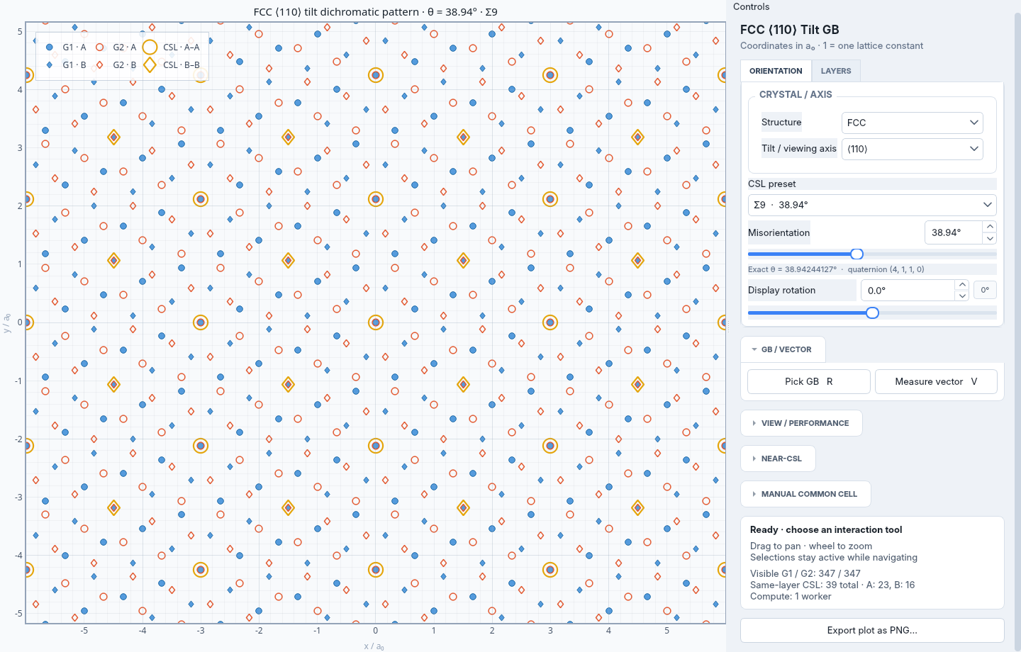
The example above shows FCC ⟨110⟩ at the Σ9 preset. The plot is on the left; settings and results are in the scrollable Controls panel on the right. Click section headers to expand them, and switch between the ORIENTATION and LAYERS tabs at the top. By default, blue markers represent G1 and orange outlines represent G2. Marker shapes distinguish axial layers, and gold outlines mark same-layer exact coincidences.
-
Choose the grains. In ORIENTATION, select Structure (
FCC,BCCorSC) and View axis, then choose a CSL preset or enter a Misorientation. For a custom axis, choose Custom [h k l], enter an integer triple such as1 -1 3, and click Apply axis or press Enter. The angle range follows the axis: 0–45° for ⟨100⟩, 0–90° for ⟨110⟩, 0–60° for ⟨111⟩, and 0–180° for other cubic axes such as ⟨112⟩. Custom indices use the same symmetry calculation; the angle field, slider and CSL presets update together. Display rotation turns the drawing without changing the grain geometry. -
Choose visible layers. Open LAYERS and toggle individual G1 A, G2 A, etc. For a first selection, click No layers, then enable G1 A and G2 A. Coincidence and local-pair markers require the layer to be visible in both grains. Enable Automatic common cell to display an available exact or strain-search cell; Fit cell frames it in the view.
-
Navigate. Drag to pan and use the wheel to zoom. Under VIEW / PERFORMANCE → VIEW, Field size selects a wider or narrower region; Center view (
C) returns to the origin at the current zoom. Grain reference axes, enabled by default, shows orientation arrows in the selected grain colors (blue G1 and orange G2 by default), sharing one fixed origin at the lower left. Color distinguishes the grains; no G1/G2 headings are drawn. Their panel keeps its size and position as the arrows rotate. They mark perpendicular reference directions and follow grain and display rotation; under strain they follow only the polar rigid rotation. The PERFORMANCE tab contains CPU workers. -
Choose colors and symbols. Open VIEW / PERFORMANCE → APPEARANCE. Click the G1 or G2 color button to choose that grain's color, and use each layer's symbol menu to choose its shape for both grains. Symbols already used by other layers are disabled. Reset appearance restores the original colors and shapes; layers beyond the first twelve use distinct numbered circles. Changes preserve selections, counts and applied strain, and appear in PNG exports.
-
Measure a vector. In GB / VECTOR, click Measure vector (
V), then click two distinct visible atom positions, P1 and P2. Read the vector annotation at the lower left of the plot, above the reference axes when they are enabled. Same-grain picks show that grain's coordinates; cross-grain picks show both G1 and G2 representations. P2 axial periodic image selects an axial repeat for the second endpoint without adding plotted atoms. -
Define a boundary. Click Pick GB (
R) and select B1, then B2. The side switches appear after the second pick; left/right are relative to B1 → B2. Use1or2for the two complementary grain-side arrangements, andFto show all sides again. Layer visibility settings still apply. -
Select and count a cell. Expand MANUAL COMMON CELL, click Pick 4 CSL vertices (
M), and select four gold sites of one layer in clockwise or counterclockwise order around a convex cell. Use Undo vertex, Clear or Fit as needed. The readout gives G1/G2 counts for the complete selected cell, including portions outside the current view. Apply GB side visibility to counts optionally restricts those counts to the displayed grain sides. -
Export the figure. Scroll to Export PNG…, choose a file name and save. The PNG contains the plot with its current layers, rotation, reference axes when enabled, and annotations; the controls are excluded.
-
Save or restore a session. Click Save session… beside Export PNG… to save one
.dmapfile containing the current structure, selections, applied strain/translations, display settings including colors and symbols, and numerical CSV tables. In ORIENTATION, use Import session… to restore it in the current window. The file is a standard ZIP archive; open it with a ZIP tool to readcounts.csv,vectors.csvandstrain.csv.
Press Esc to stop picking while retaining existing selections. Pressing R
or V starts a fresh boundary or vector selection. Click near a visible atom
or eligible cell marker; background clicks do not create arbitrary vertices.
For inexact orientations, expand NEAR-CSL, select a Method, and click Enable Near-CSL:
| Method | How to use it | Effect |
|---|---|---|
| Local matching · no bulk strain | Adjust Local pair distance; inspect purple midpoint markers and use them for manual cell picks | Finds nearby same-layer pairs while preserving the atom positions |
| Homogeneous strain + periodic cell | Set Max principal strain and Search index bound, then choose a returned candidate | Automatically applies the first result, or the candidate you select, to both grains |
A manually selected local cell containing at least one near pair can also be fitted with Apply bulk strain to selected cell in MANUAL COMMON CELL. Set its strain and rotation limits before applying; Restore original local structure returns to the original geometry. This operation has a separate apply step from the automatic search.
For control-by-control instructions, selection rules, result interpretation and troubleshooting, see the English GUI guide or 中文 GUI 使用指南. Detailed workflows cover vector measurements, Near-CSL methods, and manual cells and counts.
Python usage
from dichromatic_map import get_geometry, projected_columns, local_near_pairs

geometry = get_geometry("FCC", "110")
grain1 = projected_columns(12, 9, rotation_deg=11, lattice="FCC", axis="110")
grain2 = projected_columns(12, 9, rotation_deg=-11, lattice="FCC", axis="110")
pairs = local_near_pairs(grain1, grain2, distance=0.05)

print("Axial layers:", geometry.layer_count)
print("Near pairs:", len(pairs.layers))
print("Pair separations / a0:", pairs.distances)
The grains above have a reference misorientation of 22°. Matching uses the supplied projected columns and preserves their layer labels.
Function exported by dichromatic_map |
Purpose |
|---|---|
get_geometry |
Obtain planar geometry, axial layers and repeat distance |
misorientation_range |
Obtain the fixed-axis angle limit and rotational symmetry period |
projected_columns |
Generate a grain's projected columns in a rectangular region |
same_layer_coincidence_sites |
Locate same-layer coincidences within a specified tolerance |
local_near_pairs |
Find same-layer mutual nearest pairs within a distance threshold |
exact_csl_cell |
Obtain a layer-preserving common translation cell for a recognized commensurate angle |
count_cell_atoms |
Count atoms in complete shared or per-grain polygons |
Documentation
| Topic | English | 中文 |
|---|---|---|
| Installation, viewer workflows and Python API | User guide | 使用手册 |
| Algorithms, numerical conventions and implementation | Implementation details | 开发细节 |
Contributing and support
Report problems through GitHub Issues or yliu3500@gatech.edu. Contributions can be submitted as a pull request or by email; see the contribution guide. This project is developed by volunteers and does not currently accept external donations.
License
DichromaticMap is distributed under the MIT License.
1 maintainer

Metadata
1 maintainer
Release files for dichromatic-map 0.1.3
For a detailed explanation of source distributions (sdists) and built distributions (wheels), please see the package formats documentation.
Source distribution (sdist)
| File | Size | Uploaded | |
|---|---|---|---|
| dichromatic_map-0.1.3.tar.gz | 377.6 kB | Details |
Built distribution (wheel)
| File | Interpreter | ABI | Platform | Reset |
|---|---|---|---|---|
| dichromatic_map-0.1.3-py3-none-any.whl | Python 3 | none | any | Details |
Total release size: 477.0 kB
Release files / dichromatic_map-0.1.3.tar.gz
| Download URL | dichromatic_map-0.1.3.tar.gz |
|---|---|
| Size | 377.6 kB |
| Tags | Source |
|
SHA-256 checksum How to use checksums |
da54c0721e6414cdfaa584e07e31f90e432fbdd5b10ebf63a3f8669373121619
|
|
BLAKE2b-256 checksum How to use checksums |
17b72c5e22c0aa4415e07681ca255ff20c778f89de2928dfd3d0c689d6f7ba73
|
| Upload date | |
|
Uploaded using Trusted Publishing? What is trusted publishing? |
No |
| Uploaded via |
twine/7.0.0 CPython/3.12.14
|
Release files / dichromatic_map-0.1.3-py3-none-any.whl
| Download URL | dichromatic_map-0.1.3-py3-none-any.whl |
|---|---|
| Size | 99.4 kB |
| Tags | Python 3 |
|
SHA-256 checksum How to use checksums |
ad986b27d3df6b558cd911ef296a2f30a73cf7ed1da3473445d9984f50e55aca
|
|
BLAKE2b-256 checksum How to use checksums |
11787a22ac6b6bac1088ac16e6f5021a9fd594609318bd1375c2ae60b83a6373
|
| Upload date | |
|
Uploaded using Trusted Publishing? What is trusted publishing? |
No |
| Uploaded via |
twine/7.0.0 CPython/3.12.14
|














