




Differential-Independence Mixture Ensemble (“DIME”) MCMC sampling for Python
This is the Python implementation of the DIME sampler proposed in Ensemble MCMC Sampling for Robust Bayesian Inference (Gregor Boehl, 2022, SSRN No. 4250395). It provides the DIMEMove as a drop-in replacement for the great emcee MCMC package.
The sampler has a series of advantages over conventional samplers:
DIME MCMC is a (very fast) gradient-free global multi-start optimizer and, at the same time, a MCMC sampler that converges to the posterior distribution. This makes any posterior mode density maximization prior to MCMC sampling superfluous.
The DIME sampler is pretty robust for odd shaped, multimodal, black-box distributions.
DIME MCMC is parallelizable: many chains can run in parallel, and the necessary number of draws decreases almost one-to-one with the number of chains.
DIME proposals are generated from an endogenous and adaptive proposal distribution, thereby providing close-to-optimal proposal distributions for black box target distributions without the need for manual fine-tuning.
There is a nice set of slides on my website which explains the DIME principle.

Figure: A trimodal example distribution in 35 dimensions
There exist complementary stand-alone implementations in Julia language and in matlab.
Installation
Installing the repository version from PyPi is as simple as typing
pip install dime_samplerin your terminal or Anaconda Prompt.
Usage
The package provides a direct drop-in replacement for emcee:
import emcee
from dime_sampler import DIMEMove

move = DIMEMove()

...
def log_prob(x):
  ...
# define your density function, the number of chains `nchain` etc...
...

sampler = emcee.EnsembleSampler(nchain, ndim, log_prob, moves=move)
...
# off you go sampling
The rest of the usage is analog to emcee. See below for getting a quickstart or have a look this tutorial for details. The parameters specific to the DIMEMove are documented here.
Tutorial
Lets look at an example. Let’s define a nice and challenging distribution (it’s the distribution from the figure above):
# some import
import emcee
import numpy as np
import scipy.stats as ss
from dime_sampler import DIMEMove
from dime_sampler.test_all import _create_test_func, _marginal_pdf_test_func

# make it reproducible
np.random.seed(0)

# define distribution
m = 2
cov_scale = 0.05
weight = (0.33, .1)
ndim = 35
initvar = np.sqrt(2)

log_prob = _create_test_func(ndim, weight, m, cov_scale)
log_prob will now return the log-PDF of a 35-dimensional Gaussian mixture with three separate modes.
Next, define the initial ensemble. In a Bayesian setup, a good initial ensemble would be a sample from the prior distribution. Here, we will go for a sample from a rather flat Gaussian distribution.
# number of chains and number of iterations
nchain = ndim * 5
niter = 5000

# initial ensemble
initmean = np.zeros(ndim)
initcov = np.eye(ndim) * np.sqrt(2)
initchain = ss.multivariate_normal(mean=initmean, cov=initcov).rvs(nchain)
Setting the number of parallel chains to 5*ndim is a sane default. For highly irregular distributions with several modes you should use more chains. Very simple distributions can go with less.
Now let the sampler run for 5000 iterations.
move = DIMEMove(aimh_prob=0.1, df_proposal_dist=10)
sampler = emcee.EnsembleSampler(nchain, ndim, log_prob, moves=move)
sampler.run_mcmc(initchain, int(niter), progress=True)
The setting of aimh_prob is the actual default value. For less complex distributions (e.g. distributions closer to Gaussian) a higher value can be chosen, which accelerates burn-in. The value df_proposal_dist sets the degrees of freedom for the proposal distribution of the independence move. 10 is a sane default and it is rather unlikely that this value must be changed.
The following code creates the figure above, which is a plot of the marginal distribution along the first dimension (remember that this actually is a 35-dimensional distribution).
# import matplotlib
import matplotlib.pyplot as plt

# get elements
chain = sampler.get_chain()
lprob = sampler.get_log_prob()

# plotting
fig, ax = plt.subplots(figsize=(9,6))
ax.hist(chain[-niter//2 :, :, 0].flatten(), bins=50, density=True, alpha=0.2, label="Sample")
xlim = ax.get_xlim()
x = np.linspace(xlim[0], xlim[1], 100)
ax.plot(x, ss.norm(scale=np.sqrt(initvar)).pdf(x), "--", label="Initialization")
ax.plot(x, ss.t(df=10, loc=move.prop_mean[0], scale=move.prop_cov[0, 0] ** 0.5).pdf(x), ":", label="Final proposals")
ax.plot(x, _marginal_pdf_test_func(x, cov_scale, m, weight), label="Target")
ax.legend()
To ensure proper mixing, let us also have a look at the MCMC traces, again focussing on the first dimension.
fig, ax = plt.subplots(figsize=(9,6))
ax.plot(chain[:, :, 0], alpha=0.05, c="C0")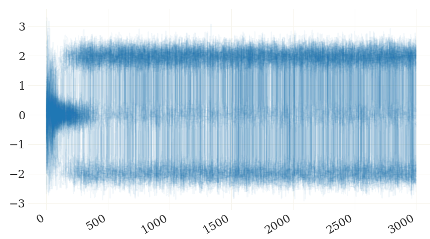
Note how chains are also switching between the three modes because of the global proposal kernel.
While DIME is an MCMC sampler, it can straightforwardly be used as a global optimization routine. To this end, specify some broad starting region (in a non-Bayesian setup there is no prior) and let the sampler run for an extended number of iterations. Finally, assess whether the maximum value per ensemble did not change much in the last few hundred iterations. In a normal Bayesian setup, plotting the associated log-likelihood over time also helps to assess convergence to the posterior distribution.
fig, ax = plt.subplots(figsize=(9,6))
ax.plot(lprob, alpha=0.05, c="C0")
ax.plot(np.arange(niter), np.max(lprob) * np.ones(niter), "--", c="C1")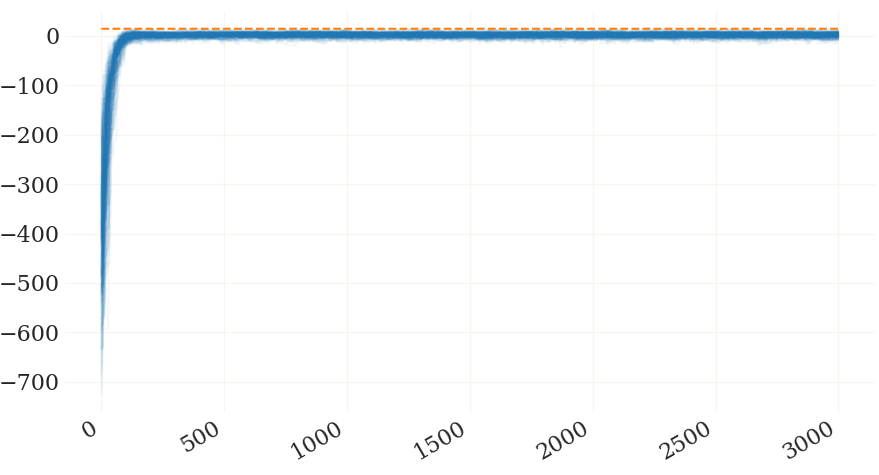
References
If you are using this software in your research, please cite
@techreport{boehl2022mcmc,
author={Gregor Boehl},
title={Ensemble MCMC Sampling for Robust Bayesian Inference},
journal={Available at SSRN 4250395},
year={2022}
}1 maintainer

Metadata
1 maintainer
Release files for dime-sampler 1.0.0
For a detailed explanation of source distributions (sdists) and built distributions (wheels), please see the package formats documentation.
Source distribution (sdist)
| File | Size | Uploaded | Provenance | |
|---|---|---|---|---|
| dime_sampler-1.0.0.tar.gz | 410.4 kB | Without provenance | Details |
Built distribution (wheel)
| File | Interpreter | ABI | Platform | Reset |
|---|---|---|---|---|
| dime_sampler-1.0.0-py3-none-any.whl | Python 3 | none | any | Details |
Total release size: 419.7 kB
Release files / dime_sampler-1.0.0.tar.gz
| Download URL | dime_sampler-1.0.0.tar.gz |
|---|---|
| Size | 410.4 kB |
| Tags | Source |
|
SHA-256 checksum How to use checksums |
160ca46c9330ef7988106e644e84d9caa0ba2b1f9d50f9bcbe50b297af954e1d
|
|
BLAKE2b-256 checksum How to use checksums |
c9f032de3bfdda83f7d82589eeb69db99c0cfe1d8b47c03821eb2c4ed0bf53ba
|
| Upload date | |
|
Uploaded using Trusted Publishing? What is trusted publishing? |
No |
| Uploaded via |
twine/5.0.1.dev0+g94f810c.d20240510 CPython/3.12.3
|
Release files / dime_sampler-1.0.0-py3-none-any.whl
| Download URL | dime_sampler-1.0.0-py3-none-any.whl |
|---|---|
| Size | 9.3 kB |
| Tags | Python 3 |
|
SHA-256 checksum How to use checksums |
d7de542372eda945bb2b00ad5c47c1b742305ec38a0727912c0067dd6502c524
|
|
BLAKE2b-256 checksum How to use checksums |
a2c22b004dc525371c441d0b743e6dd803bc6c126eb2f791b68c29d3f6e760a0
|
| Upload date | |
|
Uploaded using Trusted Publishing? What is trusted publishing? |
No |
| Uploaded via |
twine/5.0.1.dev0+g94f810c.d20240510 CPython/3.12.3
|
Security for dime-sampler 1.0.0
Provenance
Provenance describes where a file came from. On PyPI, provenance is shared via attestations, which provide a verifiable record of the build or publishing details. View details, limitations and caveats.
No provenance found
None of the files in this release were uploaded with provenance metadata.
A note on package security
PyPI is a repository for distributing packages, not a service for auditing them. While third-party security researchers and our staff do their best to detect and remove malicious packages, PyPI cannot guarantee the quality, security or suitability of any given package.
To learn more about protecting yourself from malicious actors, visit our package security documentation.














