High dimensional polytope sampling in Python with a set of tools for metabolic network sampling and analysis.

Project description

dingo is a Python package that analyzes metabolic networks.
It relies on high dimensional sampling with Markov Chain Monte Carlo (MCMC)
methods and fast optimization methods to analyze the possible states of a
metabolic network. To perform MCMC sampling, dingo relies on the C++ library
volesti, which provides
several algorithms for sampling convex polytopes.
dingo also performs two standard methods to analyze the flux space of a
metabolic network, namely Flux Balance Analysis and Flux Variability Analysis.
dingo is part of GeomScale project.


Installation
Note: Python version should be 3.8.x. You can check this by running the following command in your terminal:
python --version
If you have a different version of Python installed, you'll need to install it (start here) and update-alternatives (start here)
Note: If you are using GitHub Codespaces. Start here to set the python version. Once your Python version is 3.8.x you can start following the below instructions.
To load the submodules that dingo uses, run
git submodule update --init
You will need to download and unzip the Boost library:
wget -O boost_1_76_0.tar.bz2 https://archives.boost.io/release/1.76.0/source/boost_1_76_0.tar.bz2
tar xjf boost_1_76_0.tar.bz2
rm boost_1_76_0.tar.bz2
You will also need to download and unzip the lpsolve library:
wget https://sourceforge.net/projects/lpsolve/files/lpsolve/5.5.2.11/lp_solve_5.5.2.11_source.tar.gz
tar xzvf lp_solve_5.5.2.11_source.tar.gz
rm lp_solve_5.5.2.11_source.tar.gz
Then, you need to install the dependencies for the PySPQR library; for Debian/Ubuntu Linux, run
sudo apt-get update -y
sudo apt-get install -y libsuitesparse-dev
To install the Python dependencies, dingo is using Poetry,
curl -sSL https://install.python-poetry.org | python3 - --version 1.3.2
poetry shell
poetry install
You can install the Gurobi solver for faster linear programming optimization. Run
pip3 install -i https://pypi.gurobi.com gurobipy
Then, you will need a license. For more information, we refer to the Gurobi download center.
Unit tests
Now, you can run the unit tests by the following commands (with the default solver highs):
python3 tests/fba.py
python3 tests/full_dimensional.py
python3 tests/max_ball.py
python3 tests/scaling.py
python3 tests/rounding.py
python3 tests/sampling.py
If you have installed Gurobi successfully, then run
python3 tests/fba.py gurobi
python3 tests/full_dimensional.py gurobi
python3 tests/max_ball.py gurobi
python3 tests/scaling.py gurobi
python3 tests/rounding.py gurobi
python3 tests/sampling.py gurobi
Tutorial
You can have a look at our Google Colab notebook
on how to use dingo.
Documentation
It quite simple to use dingo in your code. In general, dingo provides two classes:
metabolic_networkrepresents a metabolic networkpolytope_samplercan be used to sample from the flux space of a metabolic network or from a general convex polytope.
The following script shows how you could sample steady states of a metabolic network with dingo. To initialize a metabolic network object you have to provide the path to the json file as those in BiGG dataset or the mat file (using the matlab wrapper in folder /ext_data to modify a standard mat file of a model as those in BiGG dataset):
from dingo import MetabolicNetwork, PolytopeSampler

model = MetabolicNetwork.from_json('path/to/model_file.json')
sampler = PolytopeSampler(model)
steady_states = sampler.generate_steady_states()
dingo can also load a model given in .sbml format using the following command,
model = MetabolicNetwork.from_sbml('path/to/model_file.sbml')
The output variable steady_states is a numpy array that contains the steady states of the model column-wise. You could ask from the sampler for more statistical guarantees on sampling,
steady_states = sampler.generate_steady_states(ess=2000, psrf = True)
The ess stands for the effective sample size (ESS) (default value is 1000) and the psrf is a flag to request an upper bound equal to 1.1 for the value of the potential scale reduction factor of each marginal flux (default option is False).
You could also ask for parallel MMCS algorithm,
steady_states = sampler.generate_steady_states(ess=2000, psrf = True,
                                               parallel_mmcs = True, num_threads = 2)
The default option is to run the sequential Multiphase Monte Carlo Sampling algorithm (MMCS) algorithm.
Tip: After the first run of MMCS algorithm the polytope stored in object sampler is usually more rounded than the initial one. Thus, the function generate_steady_states() becomes more efficient from run to run.
Rounding the polytope
dingo provides three methods to round a polytope: (i) Bring the polytope to John position by apllying to it the transformation that maps the largest inscribed ellipsoid of the polytope to the unit ball, (ii) Bring the polytope to near-isotropic position by using uniform sampling with Billiard Walk, (iii) Apply to the polytope the transformation that maps the smallest enclosing ellipsoid of a uniform sample from the interior of the polytope to the unit ball.
from dingo import MetabolicNetwork, PolytopeSampler

model = MetabolicNetwork.from_json('path/to/model_file.json')
sampler = PolytopeSampler(model)
A, b, N, N_shift = sampler.get_polytope()

A_rounded, b_rounded, Tr, Tr_shift = sampler.round_polytope(A, b, method="john_position")
A_rounded, b_rounded, Tr, Tr_shift = sampler.round_polytope(A, b, method="isotropic_position")
A_rounded, b_rounded, Tr, Tr_shift = sampler.round_polytope(A, b, method="min_ellipsoid")
Then, to sample from the rounded polytope, the user has to call the following static method of PolytopeSampler class,
samples = sample_from_polytope(A_rounded, b_rounded)
Last you can map the samples back to steady states,
from dingo import map_samples_to_steady_states

steady_states = map_samples_to_steady_states(samples, N, N_shift, Tr, Tr_shift)
Other MCMC sampling methods
To use any other MCMC sampling method that dingo provides you can use the following piece of code:
sampler = polytope_sampler(model)
steady_states = sampler.generate_steady_states_no_multiphase() #default parameters (method = 'billiard_walk', n=1000, burn_in=0, thinning=1)
The MCMC methods that dingo (through volesti library) provides are the following: (i) 'cdhr': Coordinate Directions Hit-and-Run, (ii) 'rdhr': Random Directions Hit-and-Run,
(iii) 'billiard_walk', (iv) 'ball_walk', (v) 'dikin_walk', (vi) 'john_walk', (vii) 'vaidya_walk'.
Switch the linear programming solver
We use pyoptinterface to interface with the linear programming solvers. To switch the solver that dingo uses, you can use the set_default_solver function. The default solver is highs and you can switch to gurobi by running,
from dingo import set_default_solver
set_default_solver("gurobi")
You can also switch to other solvers that pyoptinterface supports, but we recommend using highs or gurobi. If you have issues with the solver, you can check the pyoptinterface documentation.
Apply FBA and FVA methods
To apply FVA and FBA methods you have to use the class metabolic_network,
from dingo import MetabolicNetwork

model = MetabolicNetwork.from_json('path/to/model_file.json')
fva_output = model.fva()

min_fluxes = fva_output[0]
max_fluxes = fva_output[1]
max_biomass_flux_vector = fva_output[2]
max_biomass_objective = fva_output[3]
The output of FVA method is tuple that contains numpy arrays. The vectors min_fluxes and max_fluxes contains the minimum and the maximum values of each flux. The vector max_biomass_flux_vector is the optimal flux vector according to the biomass objective function and max_biomass_objective is the value of that optimal solution.
To apply FBA method,
fba_output = model.fba()

max_biomass_flux_vector = fba_output[0]
max_biomass_objective = fba_output[1]
while the output vectors are the same with the previous example.
Set the restriction in the flux space
FVA and FBA, restrict the flux space to the set of flux vectors that have an objective value equal to the optimal value of the function. dingo allows for a more relaxed option where you could ask for flux vectors that have an objective value equal to at least a percentage of the optimal value,
model.set_opt_percentage(90)
fva_output = model.fva()

# the same restriction in the flux space holds for the sampler
sampler = polytope_sampler(model)
steady_states = sampler.generate_steady_states()
The default percentage is 100%.
Change the objective function
You could also set an alternative objective function. For example, to maximize the 1st reaction of the model,
n = model.num_of_reactions()
obj_fun = np.zeros(n)
obj_fun[0] = 1
model.objective_function(obj_fun)

# apply FVA using the new objective function
fva_output = model.fva()
# sample from the flux space by restricting
# the fluxes according to the new objective function
sampler = polytope_sampler(model)
steady_states = sampler.generate_steady_states()
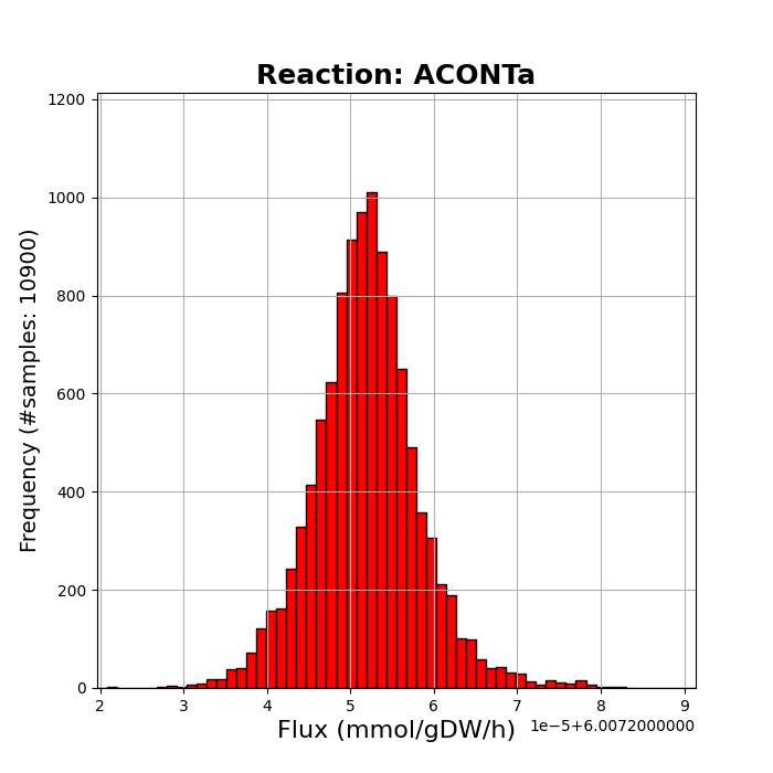
Plot flux marginals
The generated steady states can be used to estimate the marginal density function of each flux. You can plot the histogram using the samples,
from dingo import plot_histogram

model = MetabolicNetwork.from_json('path/to/e_coli_core.json')
sampler = PolytopeSampler(model)
steady_states = sampler.generate_steady_states(ess = 3000)

# plot the histogram for the 14th reaction in e-coli (ACONTa)
reactions = model.reactions
plot_histogram(
        steady_states[13],
        reactions[13],
        n_bins = 60,
        )
The default number of bins is 60. dingo uses the package matplotlib for plotting.
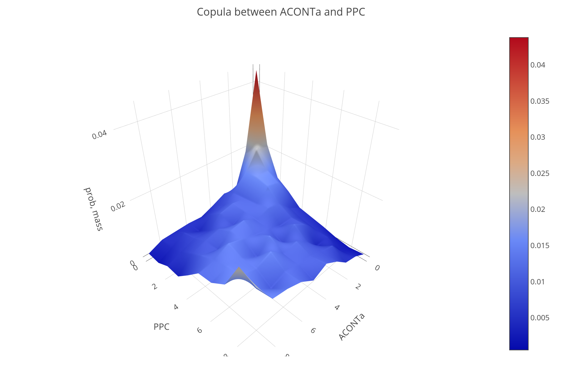
Plot a copula between two fluxes
The generated steady states can be used to estimate and plot the copula between two fluxes. You can plot the copula using the samples,
from dingo import plot_copula

model = MetabolicNetwork.from_json('path/to/e_coli_core.json')
sampler = PolytopeSampler(model)
steady_states = sampler.generate_steady_states(ess = 3000)

# plot the copula between the 13th (PPC) and the 14th (ACONTa) reaction in e-coli
reactions = model.reactions

data_flux2=[steady_states[12],reactions[12]]
data_flux1=[steady_states[13],reactions[13]]

plot_copula(data_flux1, data_flux2, n=10)
The default number of cells is 5x5=25. dingo uses the package plotly for plotting.
Release history Release notifications | RSS feed


Download files
Download the file for your platform. If you're not sure which to choose, learn more about installing packages.
Source Distribution
Built Distribution
Filter files by name, interpreter, ABI, and platform.
If you're not sure about the file name format, learn more about wheel file names.
Copy a direct link to the current filters
File details
Details for the file dingo_walk-0.1.6.tar.gz.
File metadata
- Download URL: dingo_walk-0.1.6.tar.gz
- Upload date:
- Size: 42.4 kB
- Tags: Source
- Uploaded using Trusted Publishing? No
- Uploaded via: poetry/1.3.2 CPython/3.10.13 Linux/6.8.0-57-generic
File hashes
| Algorithm | Hash digest | |
|---|---|---|
| SHA256 |
d074e2af3dc28d4cd3de650710519ff73c69428924338c3758776b46a2b479e3
|
|
| MD5 |
01cf5aaa3a331c63b9b068b26c66ad9c
|
|
| BLAKE2b-256 |
0fadbeb0b7f6a7a4e28e5052289e38a3f796460bbb7f751e5121ffd1e581e32a
|
File details
Details for the file dingo_walk-0.1.6-cp310-cp310-manylinux_2_35_x86_64.whl.
File metadata
- Download URL: dingo_walk-0.1.6-cp310-cp310-manylinux_2_35_x86_64.whl
- Upload date:
- Size: 17.0 MB
- Tags: CPython 3.10, manylinux: glibc 2.35+ x86-64
- Uploaded using Trusted Publishing? No
- Uploaded via: poetry/1.3.2 CPython/3.10.13 Linux/6.8.0-57-generic
File hashes
| Algorithm | Hash digest | |
|---|---|---|
| SHA256 |
f8d042763cd6b0ac8f24a19eef7b982d68d0efac6d9c6d79dcf40a1797dca8c6
|
|
| MD5 |
4ed64ca2f001eddfd3552d25f2b9546b
|
|
| BLAKE2b-256 |
a28398faf51074899d8cc96955d7cae0b38d69e27d6cee3c3afd233eefd72f38
|


