Deprojection Image Software for Circumstellar Objects

Project description

DISCO
Deprojection Image Software for Circumstellar Objects
A hybrid pipeline for the analysis and physical characterization of protoplanetary disks from ALMA FITS data.


⚠️ Work in Progress — DISCO is in active early development. Features and interfaces may change between releases.
Table of Contents
- Overview
- Citation
- Key Features
- Two Modes of Operation
- Installation
- GUI Workflow
- CLI Pipeline
- Tech Stack
- License
- Support & Contact
Overview
DISCO is an open-source tool for the interactive and automated analysis of protoplanetary disk observations. It combines a convolutional neural network (DiscoNet) for rapid geometric parameter prediction with a hybrid optimization strategy, enabling robust deprojection and radial profile extraction from FITS images.
DISCO bridges scientific Python libraries with a modern web interface, offering two complementary modes of operation: a GUI for interactive exploration and a CLI pipeline for reproducible batch processing.
📖 Full documentation: astrojorgeluis.github.io/disco-astronomy
Citation
If you use DISCO in published work, please cite this repository and acknowledge Jorge Luis Guzmán-Lazo, who developed the software within the YEMS Millennium Nucleus under the supervision of Sebastián Pérez and Camilo Gonzalez-Ruilova.
Key Features
- DiscoNet (CNN) — Convolutional neural network that predicts disk geometric parameters (inclination, position angle, outer/inner radius) directly from FITS images.
- Hybrid Optimization — Combines CNN predictions with fine-grained numerical refinement (Nelder-Mead) for physically consistent results.
- Dual Visualization — Real-time rendering of deprojected images in both Cartesian and polar projections.
- Batch Processing — Automated CLI pipeline supporting multiple targets and FITS files in a single run.
- Beam Homogenization — Convolves images to a common target resolution for multi-epoch or multi-band consistency (enabled by default).
- SIMBAD Metadata — Automatically queries object metadata (distance, spectral type) via the CDS SIMBAD service.
- Gaia Proper Motion Correction — Corrects source centroid across multi-epoch observations using Gaia DR3 astrometry.
- CSV Export — Outputs radial profiles and fitted parameters in tabular format.
Two Modes of Operation
| Feature | CLI Pipeline (disco-start) |
GUI (disco-start gui) |
|---|---|---|
| DiscoNet (CNN) geometry | ✅ | ❌ |
| Interactive visualization | ❌ | ✅ |
| Batch processing | ✅ | ❌ |
| Multi-band support | ✅ | ❌ |
| Beam homogenization | ✅ | ❌ |
| SIMBAD query | ❌ | ✅ |
| Session save / restore | ❌ | ✅ |
| Ease of use | Moderate | High |
The GUI is recommended for exploratory analysis and first-time users. The CLI is designed for reproducible, automated pipelines.
Installation
Recommended: Use a dedicated virtual environment to avoid dependency conflicts.
# 1. Create and activate a virtual environment
python -m venv disco-env
source disco-env/bin/activate        # Linux / macOS
disco-env\Scripts\activate           # Windows

# 2. Install DISCO from PyPI
pip install disco-astronomy

# 3. Verify the installation
disco-start --help
📦 Available on PyPI: pypi.org/project/disco-astronomy
To keep DISCO up to date:
pip install --upgrade disco-astronomy
Dependencies
All dependencies are resolved automatically by pip:
| Package | Min. Version | Role |
|---|---|---|
fastapi |
≥ 0.110.0 | HTTP backend for the GUI server |
uvicorn[standard] |
≥ 0.29.0 | ASGI server |
python-multipart |
— | File upload support |
astropy |
≥ 6.0.0 | FITS I/O, WCS, coordinate transforms |
scipy |
≥ 1.11.0 | Numerical optimization, signal processing |
matplotlib |
≥ 3.8.0 | Scientific figure rendering |
astroquery |
≥ 0.4.7 | Gaia DR3 and SIMBAD queries |
numpy |
< 2.0.0 | Array operations (pinned for compatibility) |
torch |
≥ 2.0.0 | DiscoNet CNN inference |
tqdm |
≥ 4.66.0 | CLI progress reporting |
GUI Workflow
Launch the interactive web interface with:
disco-start gui
This starts a local server at http://localhost:8000 and opens a browser tab automatically.
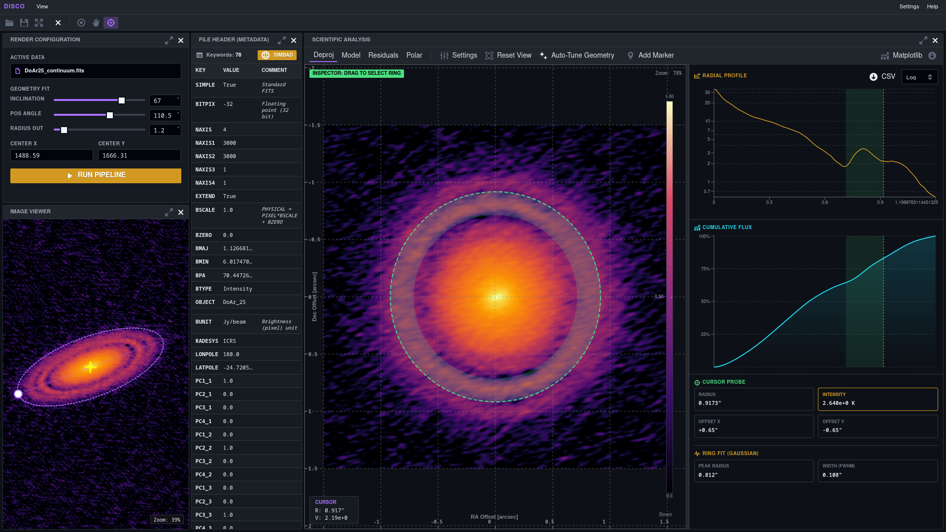
Step-by-Step Guide
A typical session follows these steps:
1. Load a FITS file
Click the folder icon in the toolbar and select your .fits file. The image will appear in the viewer and the FITS header will populate automatically in the metadata panel.
2. Adjust the disk geometry In the CONTROLS panel on the left, use the sliders to set the initial geometric parameters:
- Inclination — disk inclination in degrees (0° = face-on, 90° = edge-on).
- Position Angle — orientation of the disk major axis in degrees.
- Radius Out — estimated outer disk radius in arcseconds.
- Center X / Y — pixel coordinates of the disk center (auto-initialized to the image midpoint).
Activate the Ellipse Tool in the toolbar to display the geometry overlay on the image. As you move the sliders, the ellipse updates live so you can visually align it with the disk before running the pipeline.
3. Run the pipeline Click RUN PIPELINE. DISCO computes the deprojected image, azimuthally-averaged radial profile, cumulative flux curve, and Gaussian ring fit for the current parameters.
4. Auto-tune the geometry (optional) Click Auto-Tune Geometry in the analysis panel to run the optimizer automatically. It performs a grid-search seeded Nelder-Mead minimization of the geometric loss and applies the best-fit inclination, position angle, and center — no manual tuning required.
5. Explore the results Switch between Deproj / Model / Residuals / Polar views to inspect different representations of the disk. Activate the Inspector tool and hover over the image to probe the radial profile in real time. Drag on the profile chart to define a fitting range for Gaussian ring analysis.
6. Export Download the radial profile as CSV, save the current view as a FITS file, or open the Matplotlib Widget for a publication-ready figure. Use Save Session to preserve your parameters for later.
Toolbar Reference

The toolbar provides file management and viewer interaction controls. The active mode is highlighted with a purple background.
| Icon | Name | Description |
|---|---|---|
| 📁 | Open File | Opens a file picker to load a .fits image or a previously saved .json session file. |
| 💾 | Save Session | Saves current parameters (inclination, PA, radius, center) and the active filename to a .json file for later restoration. |
| ⛶ | Fullscreen | Expands the viewer panel to fill the browser window. |
| ✕ | Close | Clears the currently loaded file and resets the interface. |
| ◎ | Ellipse Tool | It allows you to manipulate the shape of the ellipse. The ellipse reflects the current inclination, position angle, and outer radius in real time as you adjust the sliders and/or move the ellipse control. Use it as a visual guide before running the pipeline. |
| 🖐 | Pan | Switches to pan/drag mode for navigating across large images. |
| ⊕ | Inspector | Enables the Cursor Probe. Hovering over the image synchronizes the crosshair position with the 1D radial profile chart and shows Radius, Intensity (K), and X/Y sky offsets in real time. |
View Modes
Once the pipeline has run, toggle between these representations using the tabs in the analysis panel:
| Mode | Description |
|---|---|
| Deproj | The deprojected (face-on) image computed from the current geometric parameters. |
| Model | The azimuthally-averaged synthetic model — a perfectly symmetric reconstruction of the disk. |
| Residuals | Difference between the deprojected image and the model. Highlights non-axisymmetric structures such as spirals, arcs, or clumps. |
| Polar | The deprojected image resampled into polar coordinates (Radius vs. Azimuth angle). |
Analysis Tools
Auto-Tune Geometry Runs a grid-search seeded Nelder-Mead minimization to find the optimal inclination, position angle, and center offset. Results are applied immediately to the sliders.
Gaussian Ring Fitting Click and drag on the radial profile chart to define a fitting range. The pipeline fits a Gaussian to the selected interval and reports:
- Peak Radius — centroid of the fitted Gaussian in arcsec.
- Width (FWHM) — full width at half maximum of the ring in arcsec.
Cursor Probe (Inspector) While the Inspector tool is active, hovering over the image shows:
- Radius — radial position in arcseconds.
- Intensity — brightness temperature at the nearest profile sample, in Kelvin.
- Offset X / Y — projected sky offsets in arcseconds.
Custom Markers
Click Add Marker to enter placement mode. A dialog lets you define a label, shape (circle, square, star, cross), and color. Markers are rendered as overlays on the image for the duration of the session.
SIMBAD Query Click the SIMBAD button in the metadata panel to query the CDS database for known objects near the image center (within 2 arcminutes). Returns object type, V-band magnitude, and distance.
Real-Time Charts
- Radial Profile — Intensity vs. Radius with toggleable linear / logarithmic Y-axis scaling.
- Cumulative Flux — Enclosed flux fraction as a function of radius.
Display Configuration
Click Settings in the analysis panel toolbar to access visualization controls:
| Control | Options |
|---|---|
| Colormap | magma, inferno, viridis, seismic, gray, jet (all invertible) |
| Stretch | asinh, linear, log, sqrt |
| Intensity Limits | Manual Vmin / Vmax, or Auto (percentile-based scaling) |
| Contours | Toggle on/off; configurable number of levels (1–50) |
| Overlays | Axes, colorbar, beam ellipse |
Export & Session Management
| Action | Description |
|---|---|
| Download FITS | Saves the currently displayed view (Deproj, Model, Residuals, or Polar) as a standard .fits file. |
| CSV Export | Downloads the 1D radial profile — Radius, Raw Intensity, and Brightness Temperature — as radial_profile.csv. |
| Matplotlib Widget | Opens a secondary panel with a high-DPI Matplotlib figure and configurable axes, colorbar, and beam overlay. |
| Save Session | Serializes {filename, params, pixelScale, timestamp} to a downloadable .json file. |
| Restore Session | Load a saved .json via the folder icon to resume with all parameters restored. |
CLI Pipeline
The CLI pipeline is designed for automated, reproducible processing without any browser interaction. It discovers FITS files in the working directory, groups them by source name and spectral band, and processes each group through five sequential phases: FITS reading → geometry optimization → beam homogenization → deprojection & profile extraction → output writing.
DiscoNet weights are loaded once at startup and reused across all groups. If the model file is absent, the pipeline falls back to analytical geometry optimization.
Usage Examples
# Process ALL FITS files found in the current working directory
disco-start

# Process a single object by name prefix
disco-start AS209

# Process multiple objects in one run
disco-start AS209 Elias29 DoAr25

# Process a directory group
disco-start path/to/group/

# Process a FITS file directly
disco-start path/to/disk.fits

# Force inclination and PA, export CSV and debug image
disco-start AS209 --incl 35.0 --pa 120.0 --csv on --debug on

# Set outer radius and disable beam homogenization
disco-start AS209 --rout 1.2 --homobeam off

# Specify a custom homogenization beam size
disco-start AS209 Elias29 --homobeam on --beam 0.15
If no
identifieris provided, DISCO discovers and processes all FITS files found in the current directory tree.
CLI Reference
usage: disco-start [-h] [--rout ROUT] [--rmin RMIN] [--incl INCL] [--pa PA]
                   [--beam BEAM] [--homobeam {on,off}] [--csv {on,off}]
                   [--debug {on,off}] [identifier ...]
| Argument | Default | Description |
|---|---|---|
identifier |
(all FITS in CWD) | Object name prefix(es), directory path(s), or direct .fits file path(s). |
--rout ROUT |
auto | Force outer radius in arcsec. Bypasses automatic estimation. |
--rmin RMIN |
0.0 (auto) |
Force inner radius / cavity in arcsec. When 0.0, auto-detected from beam size. |
--incl INCL |
auto | Force disk inclination in degrees. Must be paired with --pa to skip the optimization phase entirely. |
--pa PA |
auto | Force position angle in degrees. Must be paired with --incl to skip the optimization phase entirely. |
--beam BEAM |
auto | Target beam size in arcsec for homogenization. Defaults to the largest beam in the group × 1.01. |
--homobeam {on,off} |
on |
Enable / disable beam homogenization. Enabled by default. |
--csv {on,off} |
off |
Write CSV outputs: global parameters, per-band metadata, and tabulated radial profiles. |
--debug {on,off} |
off |
Save a diagnostic PNG overlaying the optimized center and outer radius on the deprojected image. |
Tech Stack
| Layer | Technology |
|---|---|
| Backend | Python 3.9+, FastAPI, Uvicorn |
| Science | Astropy, SciPy, NumPy, astroquery |
| Deep Learning | PyTorch (DiscoNet CNN) |
| Frontend | React, Vite, BlueprintJS, Recharts |
| Distribution | PyPI (disco-astronomy) |
License
This project is licensed under the MIT License.
Support & Contact
If you encounter issues or have questions, feel free to reach out:
Bug reports and feature requests are welcome via GitHub Issues.
Release history Release notifications | RSS feed


Download files
Download the file for your platform. If you're not sure which to choose, learn more about installing packages.
Source Distribution
Built Distribution
Filter files by name, interpreter, ABI, and platform.
If you're not sure about the file name format, learn more about wheel file names.
Copy a direct link to the current filters
File details
Details for the file disco_astronomy-1.2.0.tar.gz.
File metadata
- Download URL: disco_astronomy-1.2.0.tar.gz
- Upload date:
- Size: 75.3 MB
- Tags: Source
- Uploaded using Trusted Publishing? No
- Uploaded via: twine/6.2.0 CPython/3.11.15
File hashes
| Algorithm | Hash digest | |
|---|---|---|
| SHA256 |
ec22c558fd8391070c7e1f722f591ba26e3f3aa8f9629573b7a675168bd98123
|
|
| MD5 |
1a4ff1227fab1b5158dfb69477aff0fd
|
|
| BLAKE2b-256 |
6ad9a61e24040d5687882011550edb9c7b404dba0f463a07ad9512631c178b5b
|
File details
Details for the file disco_astronomy-1.2.0-py3-none-any.whl.
File metadata
- Download URL: disco_astronomy-1.2.0-py3-none-any.whl
- Upload date:
- Size: 75.3 MB
- Tags: Python 3
- Uploaded using Trusted Publishing? No
- Uploaded via: twine/6.2.0 CPython/3.11.15
File hashes
| Algorithm | Hash digest | |
|---|---|---|
| SHA256 |
288445ee7041ad2f48c5b6ff323594cb298721373318d5c76842bb1f874e627f
|
|
| MD5 |
b3495b84e20bf47a0786f8adf654a541
|
|
| BLAKE2b-256 |
8b21d7f7722a7410011e893b5e6abe63112811ebe5aa55e9b05f0d23bb46258c
|


