
Design of Experiments statistical tools

Project description
DoE Statistc (doestat.py)

A Python implementation for Design of Experiments (DOE), providing tools to optimize processes, analyze factor effects, and evaluate quality metrics in robust engineering applications.
📌 Overview
Design of Experiments (DOE) is a powerful approach for systematically planning, conducting, analyzing, and interpreting controlled tests to evaluate factor effects on responses. This package offers two distinct yet complementary methods to support experimental design and analysis:
1 - Taguchi Method:
The Taguchi approach provides a robust framework for process optimization and quality improvement. By minimizing the variability in responses and optimizing the mean performance, this method is especially effective in manufacturing, engineering, and other applied sciences. Key features include:
- Evaluation of quality metrics using Signal-to-Noise Ratios (S/N) for "Bigger is Better," "Smaller is Better," and "Nominal is Better" objectives.
- Handling of multiple responses via techniques like the Multi-Response Performance Index (MRPI).
- Visualization of factor effects, interaction graphs, and predictive capabilities for optimizing responses.
- Statistical tools such as Analysis of Variance (ANOVA) for variance decomposition and factor impact assessment.
2 - Factorial Design Analysis:
Factorial designs are fundamental for understanding the interactions and contributions of multiple factors in experimental studies. This method focuses on:
- Calculation and visualization of factorial effects, including main effects and interactions.
- Representation of effects using Gaussian-based probability plots and percentage contribution charts to reveal the most influential factors.
- Support for error estimation using t-Student distribution, enhancing the reliability of conclusions.
- Compatibility with both simple and interaction-inclusive experimental designs.
✨ Features
Key Functionalities
Taguchi Method
- Signal-to-Noise (S/N) Ratios: Evaluate quality characteristics with:
- "Bigger is better"
- "Smaller is better"
- "Nominal is better"
- Multi-Response Performance Index (MRPI): Handle multiple responses with:
- Weighted methods (
"wgt") - Envelopment methods (
"env")
- Weighted methods (
- Effect Analysis: Analyze and visualize the influence of factors and interactions.
- Interaction Checks: Display interaction graphs to identify dependencies.
- Prediction: Predict responses for specific factor combinations.
- ANOVA: Perform Analysis of Variance to understand variance contributions.
Factorial Design Analysis
- Factorial Effect Calculation: Quantify the contributions of main effects and interactions in factorial designs.
- Probability Plot Visualization: Represent effects in Gaussian-based probability plots to identify significant factors.
- Percentage Contribution Analysis: Display and quantify the relative influence of each factor or interaction on overall variability.
- Error Estimation: Compute effect errors and confidence intervals using the t-Student distribution for robustness.
- Flexible Design Support: Analyze coded factorial matrices with or without interactions.
- Regression Plot Visualization: Displays the regression plot using the provided matrix data.
- Residual Plot Visualization: Shows the residual plot for the experimental data.
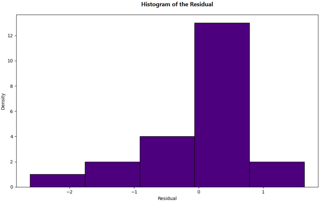
- Histogram Plot Visualization: Displays a histogram plot for the distribution of residuals.
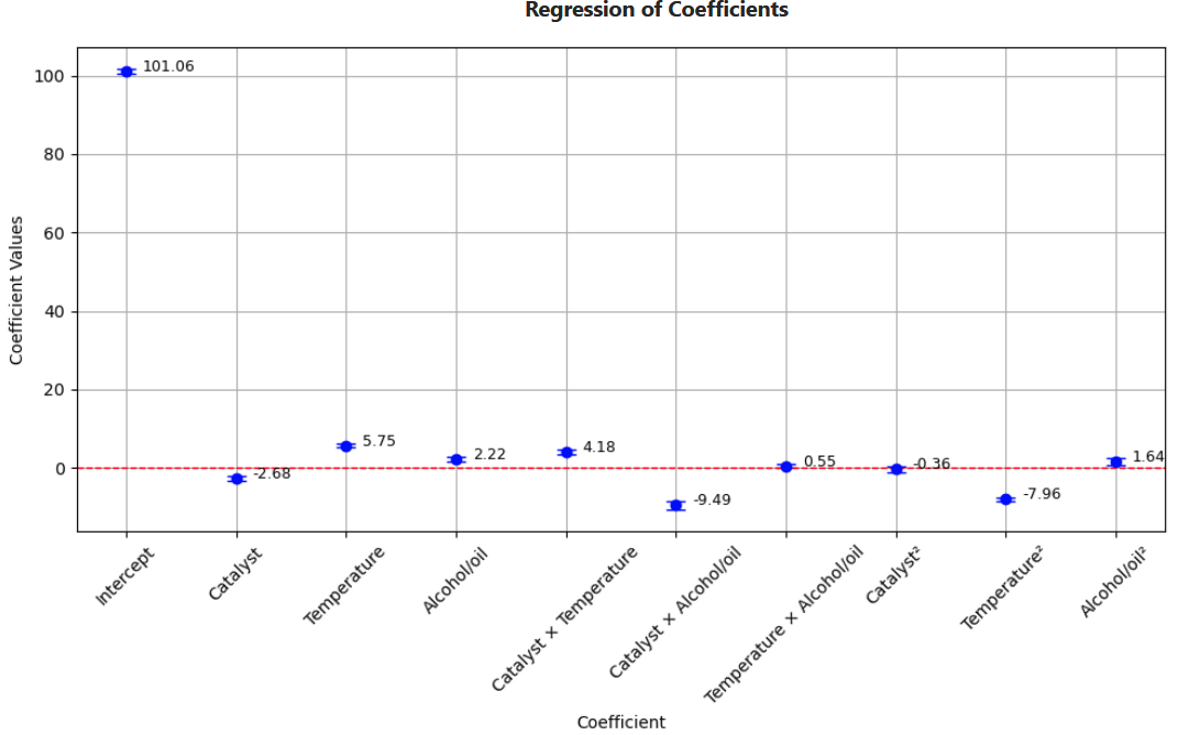
- Coefficient Error Plot Visualization: Displays the confidence intervals for the calculated regression coefficients, providing a visual representation of their variability and reliability.
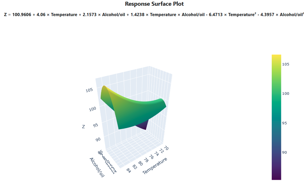
- Response Surface: Generate s surface response and contour plot with coded data or real values.
- Model Equation: Displays the model equation.
🔧 Installation
Ensure you have Python and the necessary dependencies installed. This class requires standard scientific libraries like numpy and matplotlib.
pip install pandas numpy matplotlib.pyplot plotly.graph_objs scipy.stats seaborn IPython.display sys itertools re
Recommended Stable Versions
pandas:     2.3.1
numpy:      1.26.4
matplotlib: 3.10.5
plotly:     5.24.1
scipy:      1.13.1
seaborn:    0.13.2
IPython:    8.27.0
Python:     3.12.7
Class Reference
Class: Taguchi
Parameters:
- X (matrix): Experimental design matrix containing factors (effects/interactions).
- y (array-like): Response vector or matrix. Supports single or multiple responses.
- T (float, optional): Target value for "Nominal is better" S/N ratio (default: 0).
- sn (str, optional): Quality characteristic for S/N ratio:
"max"→ Bigger is better"min"→ Smaller is better"target"→ Nominal is better
- mrpi (str, optional): Method for multi-response evaluation:
"wgt"→ Weighted method"env"→ Envelopment method
- r1, r2 (str, optional): Quality characteristics for multiple responses:
"max"→ Bigger is better"min"→ Smaller is better"target"→ Nominal is better
Attributes:
- y (array-like): Processed response vector/matrix after applying S/N ratios or MRPI.
- vector_y (array-like): Final response vector/matrix ready for analysis.
Methods:
vector_y
- Returns the processed response vector/matrix.
- Usage:
doe.Taguchi(X, y).vector_y()
effect_analysis
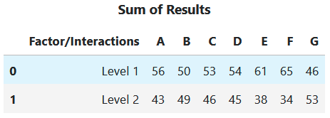
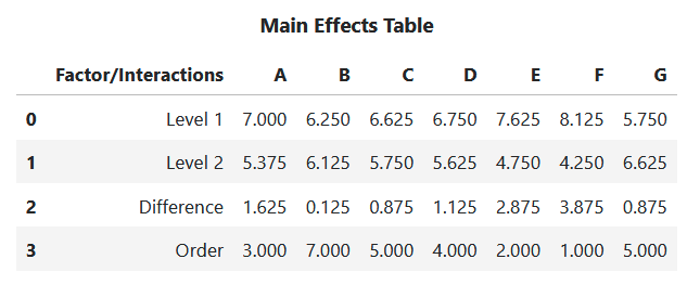
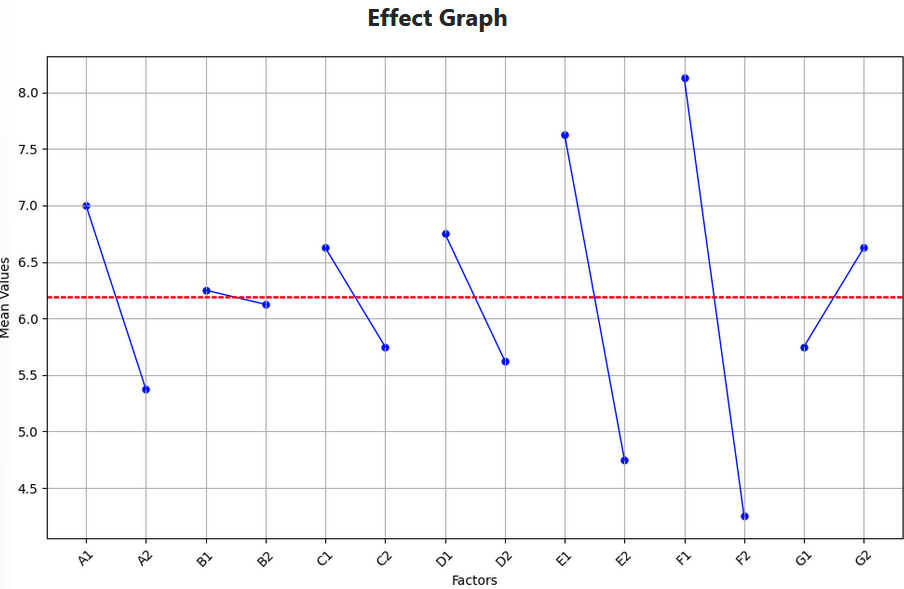
- Calculates the total response for each factor level and visualizes their effects.
- Usage:
doe.Taguchi(X, y).effect_analysis
check_interactions()
- Displays interaction graphs between selected factors.
- Usage:
doe.Taguchi(X, y).check_interactions()
prev()
- Predicts the response values for selected factors or interactions.
- Usage:
doe.Taguchi(X, y).prev()
anova()
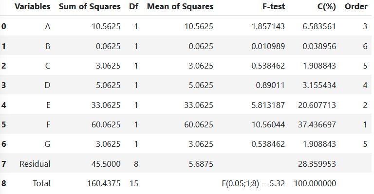
- Performs Analysis of Variance (ANOVA) and returns a summary table of variance contributions.
- Usage:
doe.Taguchi(X, y).anova()
📎 Notes
- The input data X and y must be formatted correctly:
- X: Matrix representing the experimental design.
- y: Response vector or matrix with dimensions consistent with X.
- For MRPI with multiple responses, ensure quality characteristics (r1, r2) and methods (
"wgt"or"env") are appropriately defined.
🚀 Example Usage
Here is an example to demonstrate the functionality of the Taguchi class:
df = pd.read_excel('test.xlsx', sheet_name = 'teste1')
X = df.iloc[:,1:8]
y = df.iloc[:,8:]

print('DataFrame')
print(df)
print('Matrix X')
print(X)
print('Vector y')
print(y)
DataFrame
      Exp   A  B  C  D  E  F  G  R1  R2
0        1  1  1  1  1  1  1  1  11  11
1        2  1  1  1  2  2  2  2   4   4
2        3  1  2  2  1  1  2  2   4  10
3        4  1  2  2  2  2  1  1   4   8
4        5  2  1  2  1  2  1  2   9   4
5        6  2  1  2  2  1  2  1   4   3
6        7  2  2  1  1  2  2  1   1   4
7        8  2  2  1  2  1  1  2  10   8
 Matrix X
    A  B  C  D  E  F  G
0  1  1  1  1  1  1  1
1  1  1  1  2  2  2  2
2  1  2  2  1  1  2  2
3  1  2  2  2  2  1  1
4  2  1  2  1  2  1  2
5  2  1  2  2  1  2  1
6  2  2  1  1  2  2  1
7  2  2  1  2  1  1  2
 Vector y
    R1  R2
0  11  11
1   4   4
2   4  10
3   4   8
4   9   4
5   4   3
6   1   4
7  10   8
doe.Taguchi(X,y).effect_analysis
doe.Taguchi(X,y).prev('F-1,E-1,A-1')
The predict value is:
10.38
doe.Taguchi(X,y).anova(method='Replica')
Class: Auxvalues
A auxiliar class that is used by others Classes
Class: Analysis
Parameters:
- X (matrix): Matrix representing the factors (effects/interactions) to be analyzed.
- y (array-like): Vector or matrix containing the response variable(s).
- yc (array-like, optional): Vector of central points (default: None).
- type_matrix (str, optional): Specifies if the design includes interactions to be calculated (default: None):
"interaction"
- effect_error (str, optional): Specifies the type of effect error to be considered (default: None):
"cp"→ Central Points"replica"→ Replica
Attributes:
- matrix_x (array-like): Experimental design matrix, including factors and interactions.
- vector_y (array-like): Response vector or the mean of replicates.
- error (float): Calculated effect error.
Methods:
matrix_x
- Generates design matrix, including factors and interactions
- Usage:
doe.Analysis(X, y).matrix_x
vector_y
- Show the response vector or the mean of replicates
- Usage:
doe.Analysis(X, y).vector_y
error
- Show the error effect
- Usage:
doe.Analysis(X, y).error
effect_analysis()
- Analyzes the effects of factors and optionally excludes specified variables.
- Generates:
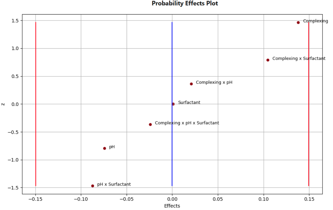
- Probability Effects Plot: Visualizes the Gaussian distribution of effects, with confidence intervals.
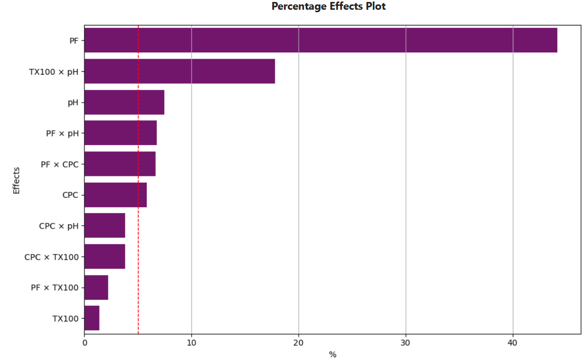
- Percentage Effects Plot: Displays the contribution of each effect to the overall variability as a horizontal bar plot.
- Usage:
doe.Analysis(X, y).effect_analysis()
📎Notes:
- This class is ideal for factorial designs and provides tools to interpret experimental results. Input Requirements:
- X: Matrix of coded factors (interactions can be generated within the class).
- y: Response vector or matrix (should be formatted appropriately).
- Effect Error and Confidence Intervals: Calculated using central points or replicates, leveraging the t-Student distribution for robustness.
- Graphs:
- Automatically saved as image files.
🚀 Examples Usage
Here is an example to demonstrate the functionality of the Analysis class:
doe.Analysis(X,y,yc,type_matrix='interaction', effect_error='cp').effect_analysis()
Class: Regression
Parameters:
- X (matrix): Matrix representing the factors (effects/interactions) to be analyzed.
- y (array-like): Vector or matrix containing the response variable(s).
- yc (array-like, optional): Vector of central points (default: None).
- type_matrix (str, optional): Specifies if the design includes interactions to be calculated (default: None):
"interaction"
- effect_error (str, optional): Specifies the type of effect error to be considered (default: None):
"cp"→ Central Points"replica"→ Replica
- selected_factors (str, optional (default=None)): Specifies the factors (effects/interactions) to be analyzed
- regression (str, optional (default = 'quadratic')): Specifies the type of regression:
"quadratic"→ Includes quadratic coefficients and, if the type_matrix='interaction', interaction coefficients."linear"→ Includes linear coefficients and, if the type_matrix='interaction', interaction coefficients.
Attributes:
-
Xb (array-like): Reorganized array for the analyzed factors.
-
Generates design matrix, including factors and interactions
-
Usage:
doe.Analysis(X, y).matrix_x
Methods:
anova
- Generates and displays a DataFrame summarizing the analysis of variance, includes results for the F-test, p-value, and evaluation of null and alternative hypotheses.
- Usage:
doe.Regression(X, y).effect_analysis()
regression_plot
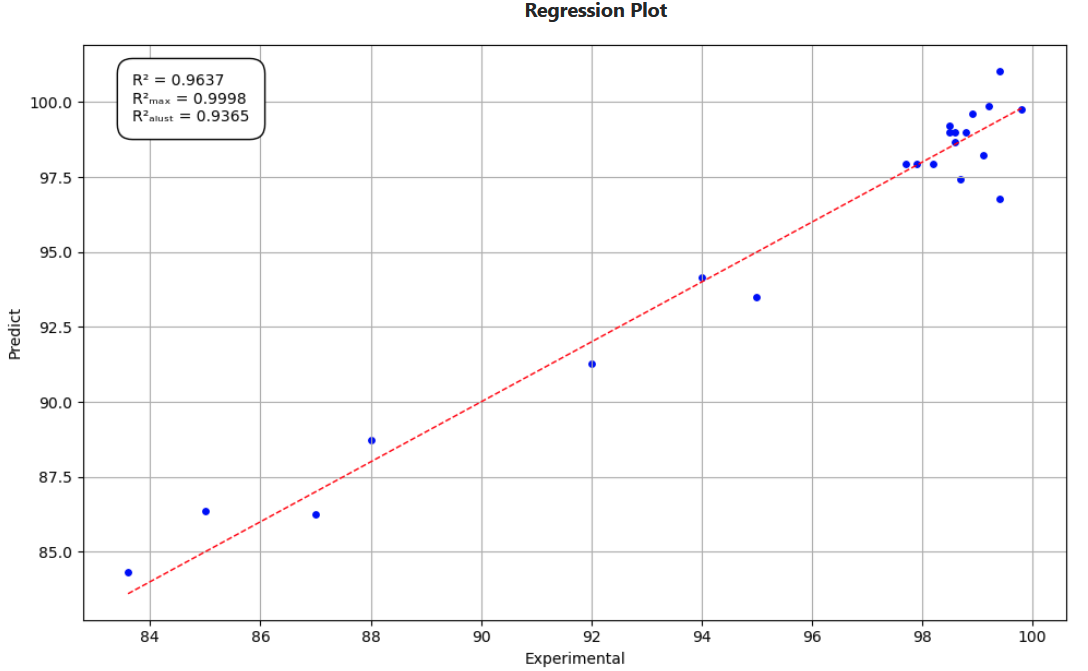
- Generates and displays the regression plot using the provided matrix data.
- Usage:
doe.Regression(X, y).regression_plot
residual_plot
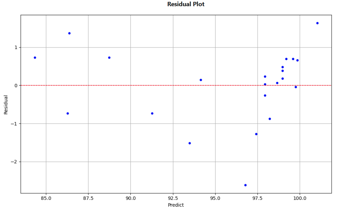
- Generates and displays the residual plot for the experimental data.
- Usage:
doe.Regression(X, y).residual_plot
histogram_plot
- Generates and displays the histogram plot for the distribution of residuals.
- Usage:
doe.Regression(X, y).histogram_plot
coefficient_error_plot
- Generates and displays the confidence intervals for the calculated regression coefficients.
- Usage:
doe.Regression(X, y).coefficient_error_plot
analysis
- Displays Regression plot, Residual plot, Histogram plot, Coefficient error plot.
- Usage:
doe.Regression(X, y).analysis
coefficient
- Generates and displays the table with the model coefficients and if their are significants.
- Usage:
doe.Regression(X, y).coefficient
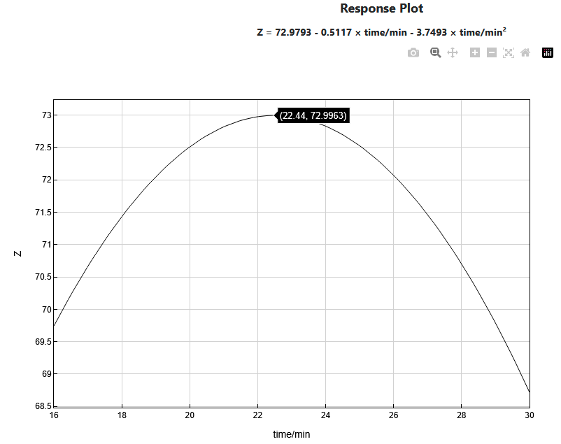
curve()
- Generates and displays a 1D graph model for better visualization.
- Usage:
doe.Regression(X, y).curve()
surface()
- Generates and displays the response surface model and corresponding contour plot or a 3D surface model for better visualization.
- Usage:
doe.Regression(X, y).surface()
show_equation()
- Displays the model equation.
- Usage:
doe.Regression(X, y).show_equation()
find_xy()
- Finds possible (x, y) values that satisfy the response surface equation for a given z.
- Usage:
doe.Regression(X, y).find_xy()
🚀 Examples Usage
Here is an example to demonstrate the functionality of the Regression class:
doe.Regression(X,y,yc, type_matrix='interaction', order=2, effect_error='cp').analysis
  v1=[70,85]
  v2=[6,13.83]
  doe.Regression(X,y,yc, type_matrix='interaction', order=2, effect_error='cp', selected_factors=['Temperature','Alcohol/oil']).surface(v1=v1,v2=v2,plot3D=True, significant_coeff=True)
  v=[16,30]
  doe.Regression(X4,yzn,yczn,effect_error='cp',regression='quadratic',selected_factors=['time/min']).curve(v=v)
📎Notes:
- This class is suitable for regression calculations in factorial designs and provides visual and numerical tools for interpreting experimental results. Input data should be formatted appropriately:
- X: should represent the coded matrix of factors. Interactions can be calculated within this class.
- y: should be the corresponding response vector or matrix.
- Graphs:
- Automatically saved as image files.
License
Copyright (C) 2025 Romulo Pires
This program is free software: you can redistribute it and/or modify it under the terms of the GNU General Public License as published by the Free Software Foundation, either version 3 of the License, or any later version.
This program is distributed in the hope that it will be useful, but WITHOUT ANY WARRANTY; without even the implied warranty of MERCHANTABILITY or FITNESS FOR A PARTICULAR PURPOSE. See the GNU General Public License for more details.
You should have received a copy of the GNU General Public License along with this program. If not, see https://www.gnu.org/licenses/.
Release history Release notifications | RSS feed

Download files
Download the file for your platform. If you're not sure which to choose, learn more about installing packages.
Source Distribution
Built Distribution
Filter files by name, interpreter, ABI, and platform.
If you're not sure about the file name format, learn more about wheel file names.
Copy a direct link to the current filters
File details
Details for the file doestat-0.1.0.tar.gz.
File metadata
- Download URL: doestat-0.1.0.tar.gz
- Upload date:
- Size: 27.6 kB
- Tags: Source
- Uploaded using Trusted Publishing? No
- Uploaded via: twine/6.2.0 CPython/3.12.1
File hashes
| Algorithm | Hash digest | |
|---|---|---|
| SHA256 |
f6e104c9c3e6c566fea03b52d94e4027027a48df46b4f250b63b2169321bddf1
|
|
| MD5 |
db403e32ad3cc0f3bbeb6e95b7a8cae3
|
|
| BLAKE2b-256 |
a61a1d52ebd0fc2e636108897d7a1c08ff31fd7005b07a62a6d088b137ed9e5a
|
File details
Details for the file doestat-0.1.0-py3-none-any.whl.
File metadata
- Download URL: doestat-0.1.0-py3-none-any.whl
- Upload date:
- Size: 27.6 kB
- Tags: Python 3
- Uploaded using Trusted Publishing? No
- Uploaded via: twine/6.2.0 CPython/3.12.1
File hashes
| Algorithm | Hash digest | |
|---|---|---|
| SHA256 |
e725c7dcb049431c65c8f6a7013cbff495f5c6f3f4492aa1799229cb73dd9bbf
|
|
| MD5 |
566f4cd5d16a2914da87e302d10d36f9
|
|
| BLAKE2b-256 |
b1366fc01bdcb25d8159bdd9cb8afd60510283c46fd19ce99bb10c231d5eadab
|






