
DRGCT
Deep-learning based doubly robust test for Granger causality — a complete, documented Python library.





drgct implements the test proposed in
Hui, Y., Liu, C. and Song, X. (2025). Deep learning based doubly robust test for Granger causality. arXiv:2509.15798v2 [stat.ME]
faithfully and completely: Algorithm 1 in full, all six simulation designs of Section 4, the three-market price–volume application of Section 5, the smoothing-based benchmark the paper compares against, and a set of journal-quality tables and figures that come out as LaTeX, Markdown, CSV, PDF and PNG in a single call.
📘 New to the method? Start with the Applied Researcher's Guide.
It walks you from a raw CSV to a finished results section, with complete runnable code at every step, and a write-up template at the end.
Table of contents
- Why this test
- Installation
- Sixty seconds
- What is in the box
- The method in one screen
- Reproducing the paper
- Real economic data
- Results gallery
- The one caveat you must not skip
- API at a glance
- Command line
- Documentation
- Honest differences from the paper
- Testing and development
- Citation
- License
Why this test
Granger causality has a standing dilemma. The linear VAR F-test is cheap and well behaved but blind to nonlinearity. Kernel-smoothing nonparametric tests see nonlinearity but collapse under the curse of dimensionality: past two or three lags they lose size control, lose power, and become hostage to a bandwidth choice. Yet economic mechanisms — monetary policy, credit transmission, investor reaction to sustained price moves — routinely operate with long and variable lags.
The DRGCT resolves the dilemma by putting deep networks inside a classical testing framework, and by using a doubly robust moment condition so that the networks' slow convergence rates multiply into a fast enough product.
| Linear VAR F | Kernel/smoothing (NHKJ class) | DRGCT | |
|---|---|---|---|
| Detects nonlinear causality | ✗ | ✓ | ✓ |
| Usable at lag 5–10 | ✓ | ✗ | ✓ |
| Bandwidth to tune | – | yes, and it matters | none |
| Size control at large lag | ✓ | badly undersized | ✓ |
| Local power rate | n^{-1/2} |
slower (smoothing) | n^{-1/2} |
| Cost per test | ms | s | s to tens of s |
From the paper's Table 3, at nominal 5% and n = 2000 with 5 lags, the
smoothing benchmark has empirical size 0.007; the DRGCT has 0.056.
From Table 4, at n = 500 with 5 lags in design P2, the benchmark's power is
0.052 — indistinguishable from the nominal level — against the DRGCT's
0.546.
Installation
pip install "drgct[data] @ git+https://github.com/merwanroudane/DRGCT.git"
From a clone, for development:
git clone https://github.com/merwanroudane/DRGCT.git
cd DRGCT
pip install -e ".[data,dev]"
drgct info
Requirements — Python ≥ 3.9, numpy, scipy, pandas, matplotlib,
torch, statsmodels, tabulate. The optional [data] extra adds
yfinance for refreshing the bundled market data.
No GPU needed — the networks are small enough that CPU is faster.
Sixty seconds
import numpy as np
from drgct import drgc_test

rng = np.random.default_rng(0)
n = 600

# X is an AR(1).  Y depends on X only through sin(.), so the linear
# projection of Y on lagged X is essentially zero: a VAR F-test sees nothing.
x = np.zeros(n); y = np.zeros(n)
e1, e2 = rng.normal(0, 0.7, n), rng.normal(0, 0.7, n)
for t in range(1, n):
    x[t] = -0.5 * x[t - 1] + e1[t]
    y[t] = 0.5 * y[t - 1] + np.sin(-x[t - 1]) + e2[t]

drgc_test(x, y, lag=1, seed=1).print()
========================================================================
  Doubly Robust Granger Causality Test (DRGCT)
  Hui, Liu & Song (2025), arXiv:2509.15798 -- Algorithm 1
========================================================================
  H0 : X does not Granger-cause Y in mean
  Construction        : doubly robust
  Lag orders          : p = 1 (cause), q = 1 (effect)
  Sample              : n = 600,  effective n - q = 599
  MDN components G    : 10
  (mu, nu) pairs L    : 20   drawn U[-1.0, 1.0]
  Pseudo-samples M    : 20
  Bootstrap B         : 1000   multipliers: rademacher
  Network (MLP/MDN)   : width 5/5, depth 1/1
------------------------------------------------------------------------
  KS_n statistic      : 8.271043
  Bootstrap p-value   : 0.0000 ***
  Critical values     : 1%: 1.7654  5%: 1.5361  10%: 1.4224
  Decision at 5%      : REJECT H0
------------------------------------------------------------------------
Scan every lag, both directions, and get a tidy table:
from drgct import drgc_lag_scan

scan, results = drgc_lag_scan(x, y, lags=range(1, 11), seed=1)
print(scan[["lag", "ks_stat", "pvalue", "reject"]].to_string(index=False))
What is in the box
DRGCT/
├── src/drgct/
│   ├── core.py           # Algorithm 1: the test, lag scans, stability check
│   ├── nets.py           # MLP (conditional mean) + MDN (conditional density)
│   ├── nhkj.py           # smoothing-based nonparametric benchmark
│   ├── dgp.py            # the six designs of Table 1, coefficients of Table 2
│   ├── simulate.py       # parallel Monte Carlo -> Tables 3 and 4
│   ├── datasets.py       # bundled market data + the Section 5 transformation
│   ├── applications.py   # the 180-test price-volume grid, rolling windows
│   ├── tables.py         # LaTeX (booktabs) / Markdown / CSV builders
│   ├── plots.py          # thirteen journal-quality figures
│   ├── cli.py            # `drgct test | simulate | app | info`
│   └── data/             # spx500.csv, csi300.csv, nikkei225.csv + SOURCES.md
├── docs/
│   ├── GUIDE.md          # ★ the applied researcher's guide, start here
│   ├── SYNTAX.md         # complete API reference
│   ├── THEORY.md         # equation-by-equation map, paper -> code
│   └── FAQ.md
├── examples/             # four runnable scripts, quick start to full study
├── scripts/              # run_simulation.py, run_application.py
├── data/fetch_data.py    # refresh or extend the bundled CSVs
├── results/              # the tables and figures shipped with the repo
└── tests/                # pytest suite
The method in one screen
Let W_{t−1} = (X_{t−1},…,X_{t−p}, Y_{t−1},…,Y_{t−q})' and
m(Y_{t−1}) = E[Y_t | Y_{t−1},…,Y_{t−q}]. The null is
H0 : E[ Y_t − m(Y_{t−1}) | W_{t−1} ] = 0 (X does not Granger-cause Y in mean)
Using the generically comprehensively revealing family exp(i·w′W)
(Stinchcombe and White, 1998) and then the doubly robust rewriting proved
equivalent in Proposition 1 of the paper:
H0 : E[ (Y_t − m(Y_{t−1})) · e^{i μ′Y_{t−1}} · ( e^{i ν′X_{t−1}} − φ(ν | Y_{t−1}) ) ] = 0
where φ(ν | Y_{t−1}) = E[e^{i ν′X_{t−1}} | Y_{t−1}]. Estimate m with an
MLP and φ with a mixture density network, evaluate
Ŝ_n(μ_ℓ, ν_ℓ) = (n−q)^{-1/2} Σ_t (Y_t − m̂) e^{i μ_ℓ′Y_{t−1}} ( e^{i ν_ℓ′X_{t−1}} − φ̂ )
KS_n          = max_ℓ max( |Re Ŝ_n| , |Im Ŝ_n| )
at L random directions, and take critical values from a multiplier
bootstrap.
Why the − φ̂ term is the whole point. Without it, the bias of the
process is first order in the MLP error and the test has no valid null
distribution. With it, the bias depends on the product ‖m̂ − m‖ ·
‖φ̂ − φ‖, so two estimators each converging slower than n^{-1/2} still
deliver a valid test. You can run the naive version yourself and watch its
size break — in our implementation it breaks downwards rather than upwards,
see results/README.md:
drgc_test(x, y, lag=5, doubly_robust=False) # the naive plug-in of equation (5)
Why the bootstrap is free. Only the multipliers ξ_t are redrawn — the
two networks are trained exactly once per test. With n = 750, L = 20,
B = 999, the bootstrap costs about 15 ms against roughly 10 s for the
networks. So never economise on B.
Full derivation and a line-by-line source map: docs/THEORY.md.
Reproducing the paper
Every table and figure in the paper has a builder.
| Paper | What it is | How to get it |
|---|---|---|
| Table 1 | The six data generating processes | drgct.tables.table_dgp_definitions() |
| Table 2 | Coefficients by lag order | drgct.tables.table_parameter_settings() |
| Table 3 | Empirical sizes | drgct.tables.table_size(mc) |
| Table 4 | Empirical powers | drgct.tables.table_power(mc) |
| Table 5 | Price–volume detection | drgct.tables.table_detection(app) |
| Table 6 | Detection by lag order | drgct.tables.table_lag_orders(app) |
| Algorithm 1 | The test | drgct.drgc_test |
# Section 4 -- Monte Carlo, Tables 3-4, size/power/p-value-plot figures
python scripts/run_simulation.py --reps 1000 --ns 500 1000 2000 -B 1000 --jobs 10

# Section 5 -- the 180-test price-volume grid, Tables 5-6, all figures
python scripts/run_application.py --jobs 10 --rolling --stability-draws 30

# two-minute plumbing checks
python scripts/run_simulation.py --quick
python scripts/run_application.py --quick
Size and power reproduce closely
A 120-replication calibration run at n = 500 against the paper's own numbers
(nominal level 5%):
| Design | lag | Paper (1000 reps) | drgct (120 reps) |
|---|---|---|---|
| S1 (size) | 1 | 0.051 | 0.058 |
| S1 (size) | 3 | 0.046 | 0.050 |
| S1 (size) | 5 | 0.050 | 0.058 |
| S2 (size) | 1 | 0.046 | 0.050 |
| S2 (size) | 3 | 0.045 | 0.067 |
| S2 (size) | 5 | 0.051 | 0.050 |
| P2 (power) | 1 | 0.996 | 1.000 |
| P2 (power) | 3 | 0.898 | 0.967 |
| P2 (power) | 5 | 0.546 | 0.583 |
| P3 (power) | 1 | 1.000 | 1.000 |
| P3 (power) | 3 | 0.954 | 0.958 |
| P3 (power) | 5 | 0.407 | 0.392 |
Every difference is within about two Monte-Carlo standard errors
(≈ 0.02 for size at 120 replications). The full run shipped in results/ uses
more replications and adds the naive plug-in and the smoothing benchmark; see
results/README.md.
Real economic data
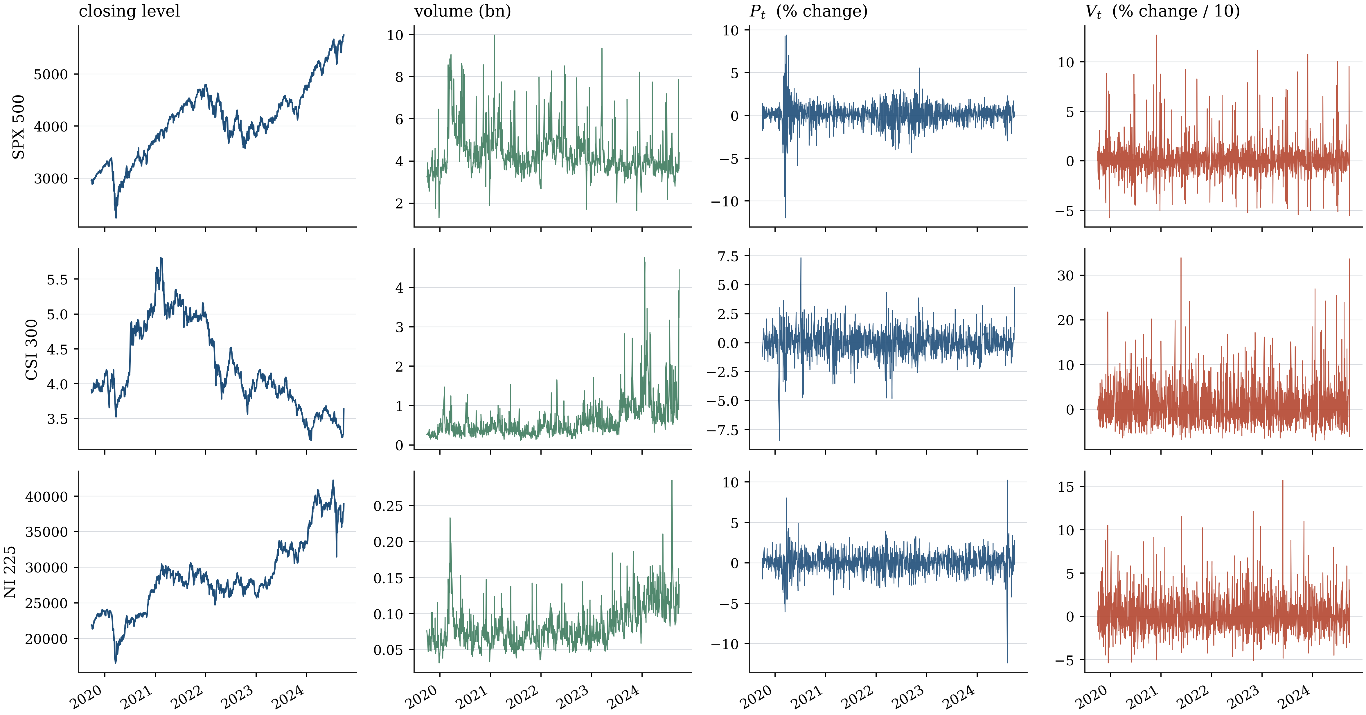
Three daily index series covering the paper's exact window, 27 September 2019 – 26 September 2024, ship inside the package so every example runs offline:
| Key | Index | Source ticker | Observations |
|---|---|---|---|
spx500 |
S&P 500 | ^GSPC |
1257 — exactly the paper's T = 1257 |
csi300 |
CSI 300 (exchange-traded tracker) | 510300.SS |
1211 |
nikkei225 |
Nikkei 225 | ^N225 |
1220 |
from drgct.datasets import load_index, to_percentage_changes, subsample

spx = load_index("spx500")                    # Date-indexed: Close, Volume
pv  = to_percentage_changes(spx)              # P = % price change,  V = % volume change / 10
sub = subsample(pv, "2021-2024")              # one of the paper's three windows
Refresh them, extend the window, or add your own tickers:
python data/fetch_data.py
python data/fetch_data.py --start 2005-01-01 --end 2024-12-31
python data/fetch_data.py --tickers ^FTSE=ftse100 ^GDAXI=dax
Provenance is recorded in
src/drgct/data/SOURCES.md. Yahoo! Finance
truncates the CSI 300 index series (000300.SS) to roughly the last three
years, so the largest exchange-traded tracker is used instead; the downloader
tries the index first and records which source it used. Drop in your own
vendor's CSV with Date, Close, Volume columns and everything runs unchanged.
Using entirely different data is one line:
import pandas as pd
panel = pd.read_csv("my_macro.csv", index_col=0, parse_dates=True).dropna()
drgc_test(panel["m2_growth"].to_numpy(), panel["cpi"].to_numpy(), lag=12, seed=1).print()
Results gallery
All figures below are in results/figures/, produced by the two scripts in
scripts/, unedited. Vector PDFs sit next to every PNG.
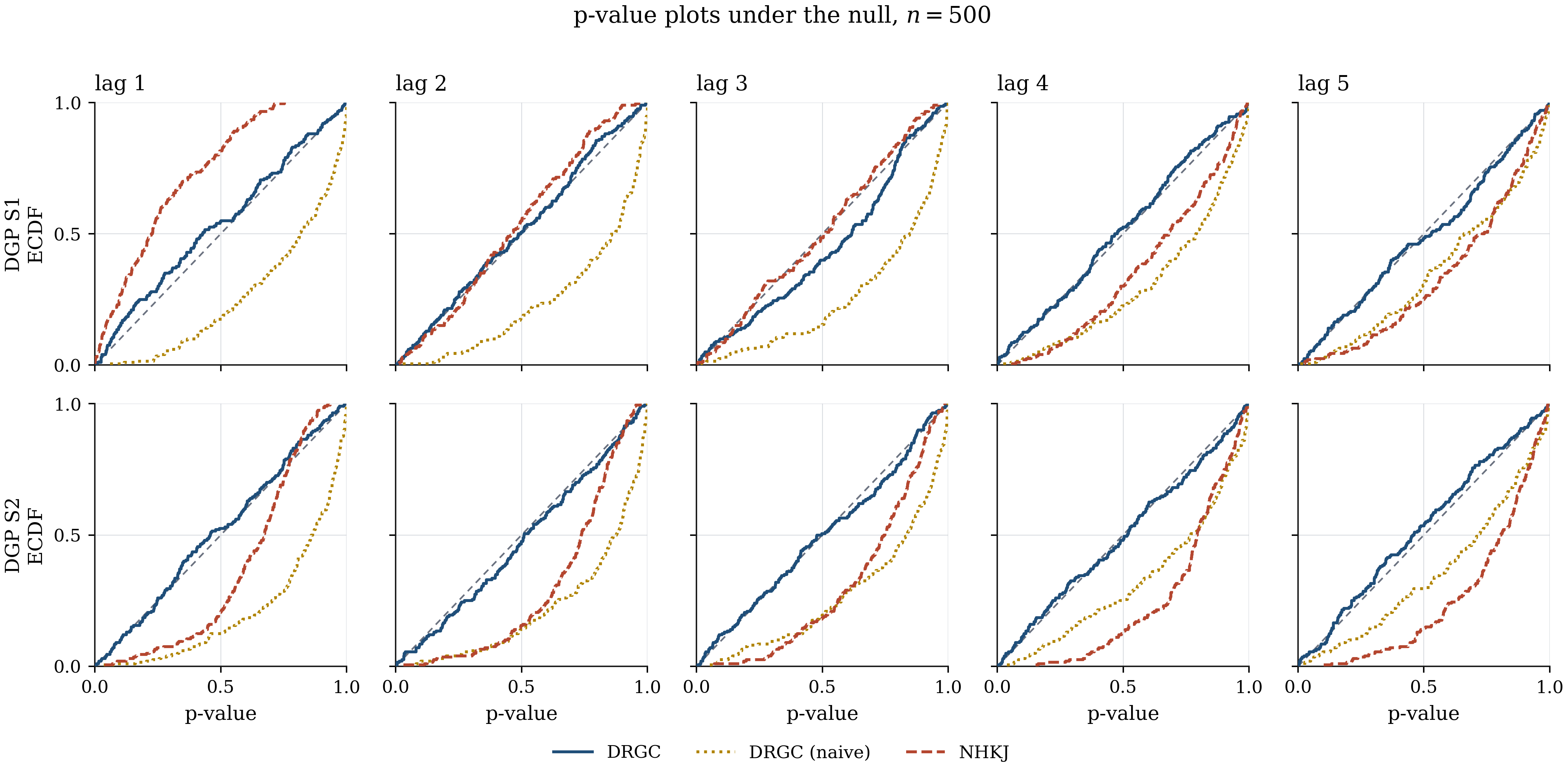
The headline simulation result: the p-values are uniform under the null
Empirical CDF of the bootstrap p-value across 200 replications of the two null
designs, n = 500. The doubly robust test (blue) sits on the 45-degree line at
every lag order — correct size. The naive plug-in (gold) and the smoothing
benchmark (red) do not.
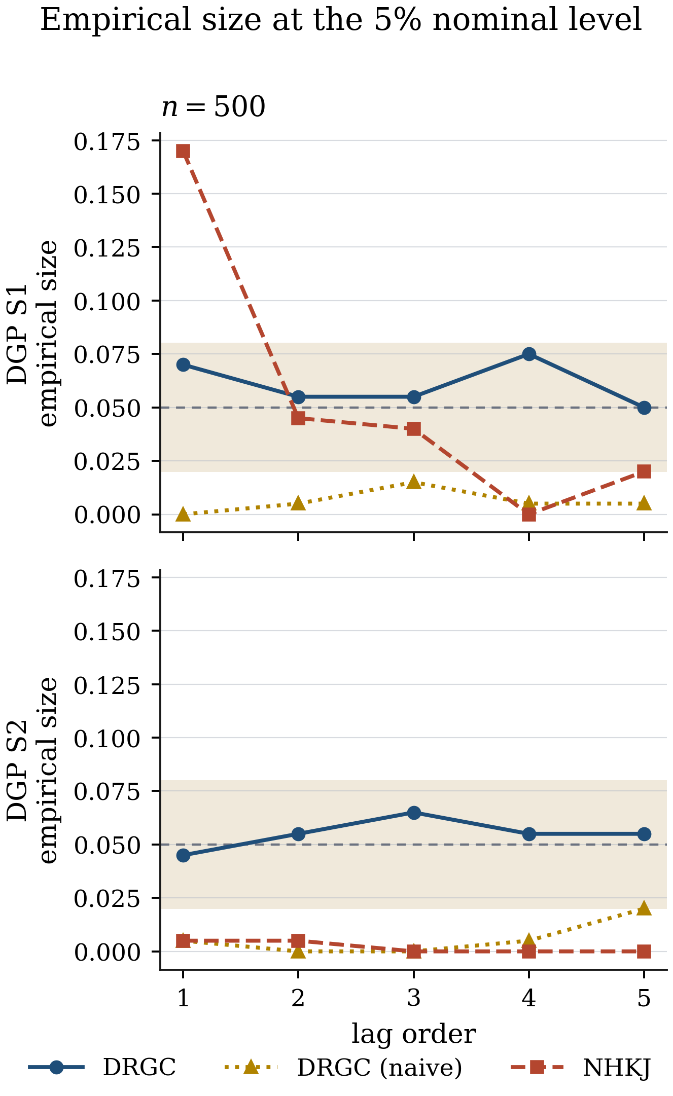
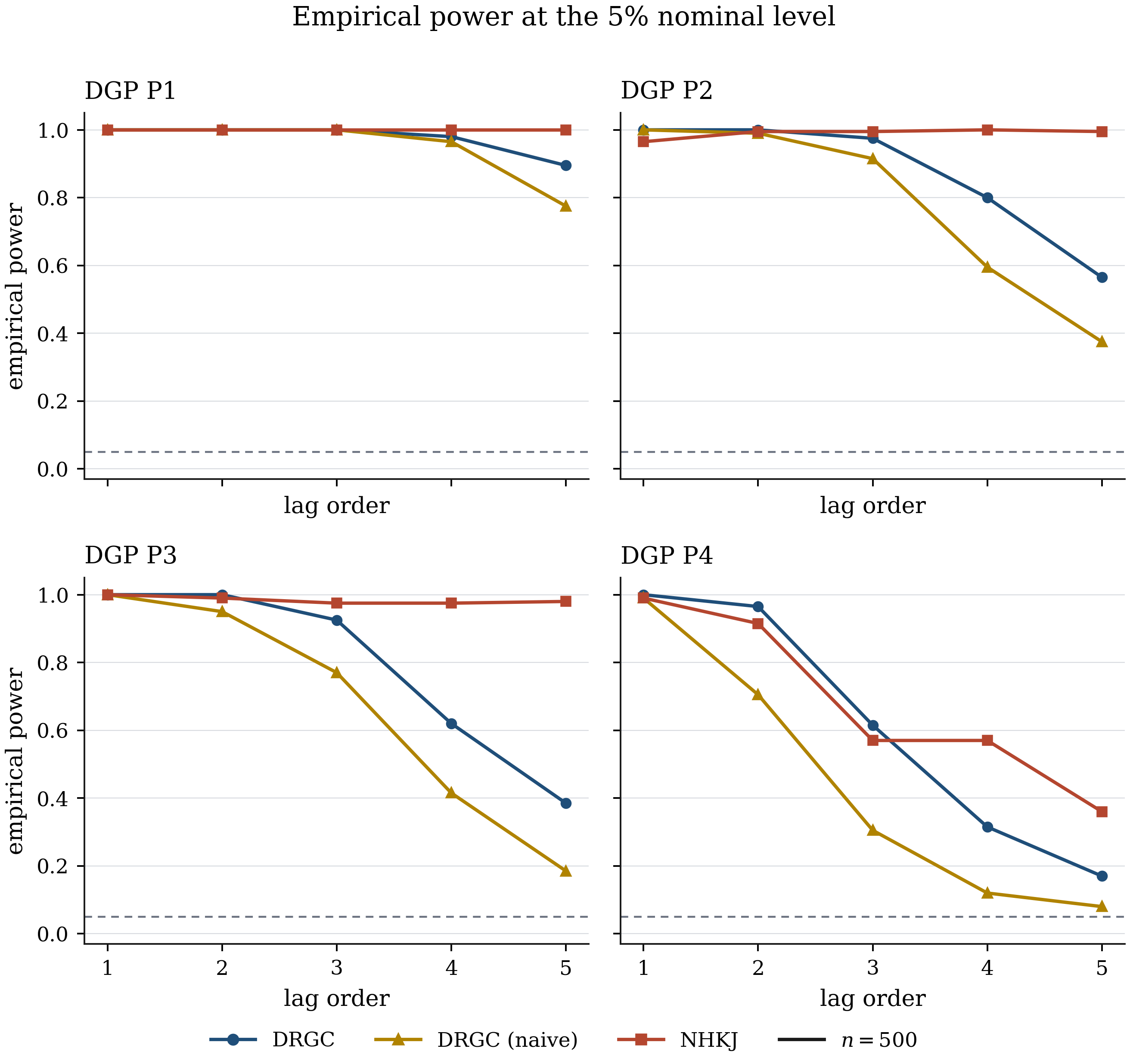
Size and power against the lag order
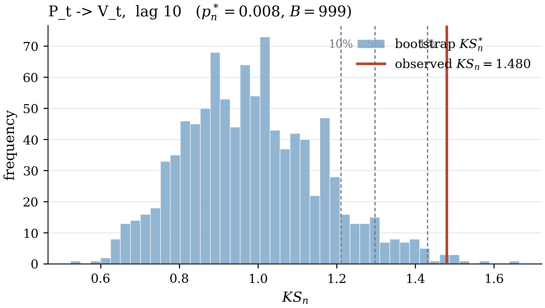
Bootstrap null distribution — makes any single p-value auditable
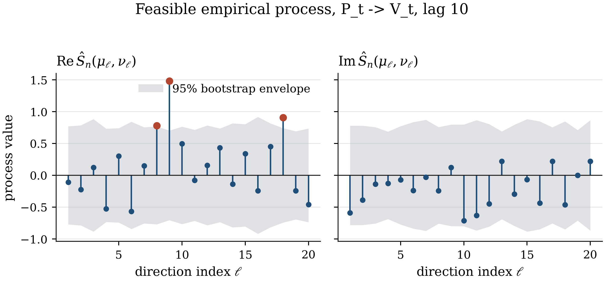
The empirical process across the L random directions
Which direction in W drives the rejection? Here exactly one of twenty
escapes the bootstrap envelope — a warning sign, and the reason for the
stability check below.
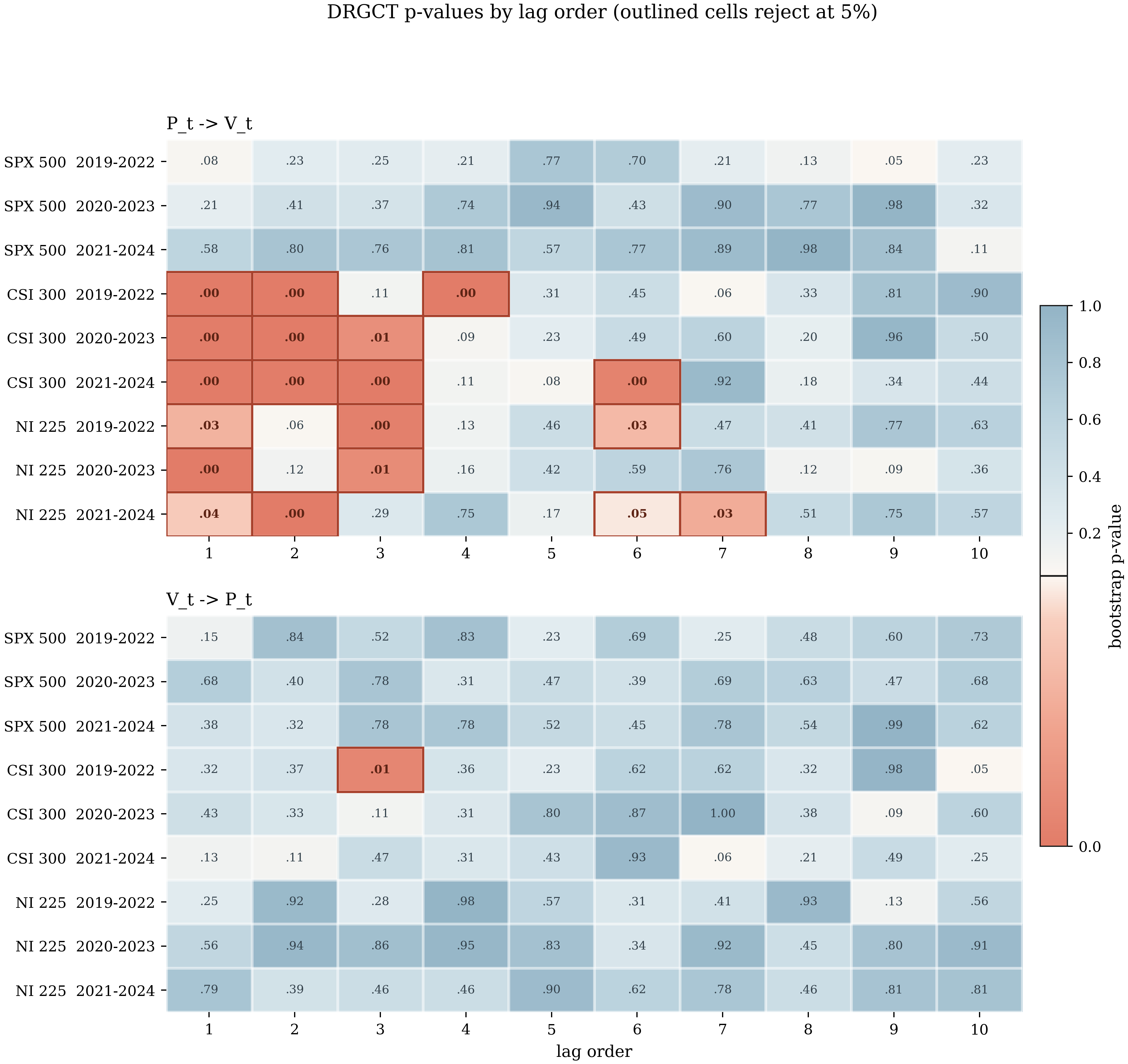
p-values across lag orders, indices and sub-samples — Table 6 as a picture
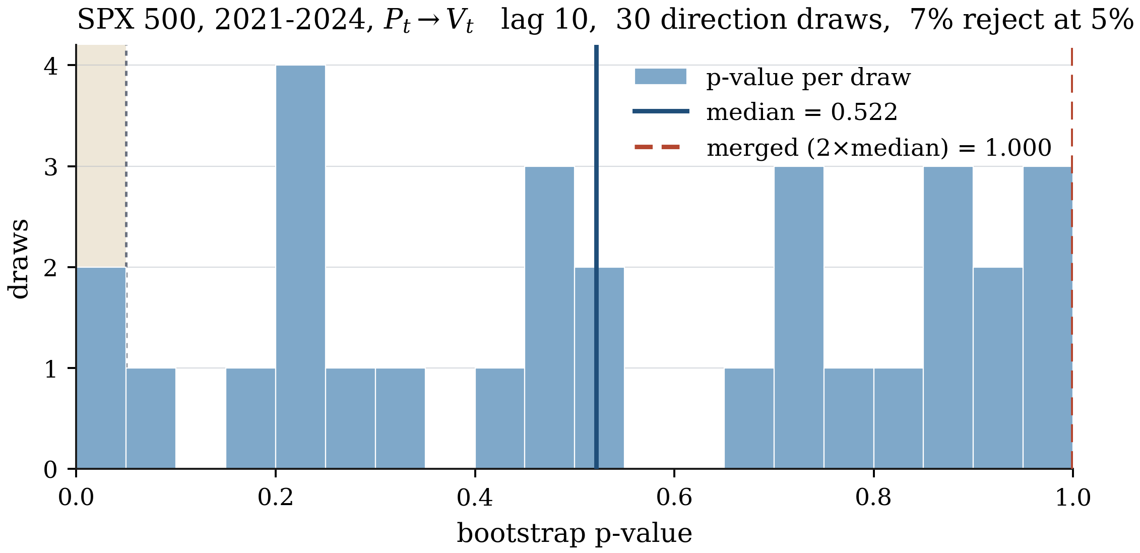
Is the conclusion an artefact of the random directions?
The data
Rolling-window causality — when does it switch on?
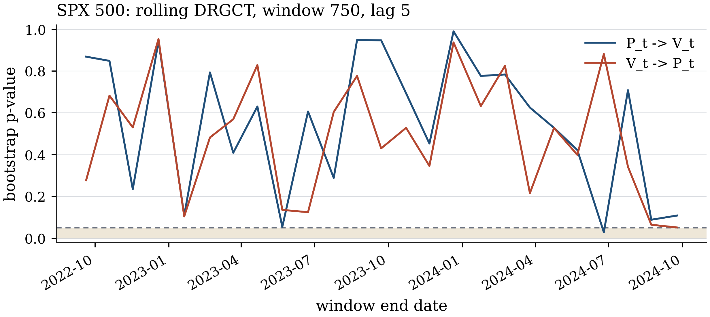
Also available: plot_size, plot_power, plot_pvalue_ecdf (the
Davidson–MacKinnon p-value plot), plot_lag_profile, plot_mdn_fit and
plot_training_curves. See docs/SYNTAX.md.
The one caveat you must not skip
Step 2(d) of Algorithm 1 draws the L evaluation directions at random.
Every draw is a valid test, but with L = 20 in a 20-dimensional conditioning
space, the draws differ enough that the p-value carries simulation noise on
top of sampling noise.
This is not hypothetical. In the bundled application, one seed put the
S&P 500 lag-10 test at p = 0.008; across 30 independent draws the median was
0.52 and only 7% of draws rejected. Reporting the first number alone
would have been badly misleading.
from drgct import drgc_stability

stab = drgc_stability(P, V, lag=10, n_draws=30, seed=1)
stab["median"]          # 0.522
stab["q05"], stab["q95"]# 0.048, 0.974
stab["share_reject"]    # 0.067
stab["merged_pvalue"]   # 1.000  -- min(1, 2 x median), valid under arbitrary dependence
Three remedies, in order: raise L (it is nearly free and also raises
power); report the distribution, not one draw; quote merged_pvalue,
which is min(1, 2 × median) and is a valid — conservative — p-value by
Rüger's inequality (see Vovk and Wang, 2020, on p-value merging).
This diagnostic is an addition to the paper, not part of it. It exists because running the method at scale on real data made the issue impossible to ignore.
API at a glance
from drgct import (
    drgc_test, drgc_lag_scan, drgc_both_directions, drgc_stability,  # the test
    nhkj_test,                                                        # benchmark
    simulate_dgp, monte_carlo, summarize, size_power_tables,          # Section 4
    load_index, to_percentage_changes, subsample, describe,           # data
    price_volume_study, rolling_causality, lag_scan_frame,            # Section 5
    MLPConfig, MDNConfig, check_stationarity, set_seed,               # config
    tables, plots,                                                    # output
)
| Task | Call |
|---|---|
| One test | drgc_test(x, y, lag=5, seed=1) |
| Both directions | drgc_both_directions(x, y, lag=5) |
| Scan lags 1–12 | drgc_lag_scan(x, y, lags=range(1, 13)) |
| Different lags per series | drgc_test(x, y, p=12, q=6) |
| Robustness to the direction draw | drgc_stability(x, y, lag=5, n_draws=30) |
| Reproduce the naive-plug-in failure | drgc_test(..., doubly_robust=False) |
| Smoothing benchmark | nhkj_test(x, y, lag=5) |
| Simulate a paper design | simulate_dgp("P2", n=500, lag=3, rng=0) |
| Full Monte Carlo | monte_carlo(reps=1000, n_jobs=-1) |
| The 180-test application | price_volume_study(n_jobs=-1) |
| Rolling windows | rolling_causality(x, y, window=750, step=21) |
| LaTeX + Markdown + CSV in one call | tables.export_table(df, "name", caption=..., label=...) |
| PDF + PNG in one call | plots.save_figure(fig, "name") |
The six knobs that matter, with the paper's values as the defaults:
| Knob | Default | Raise it when |
|---|---|---|
G — MDN mixture components |
10 | p ≥ 5; too small inflates the type I error |
L — random directions |
20 | p + q ≥ 10; cheapest available power gain |
M — pseudo-samples |
20 | p ≥ 5 |
B — bootstrap draws |
1000 | never economise; it is free |
mlp=, mdn= |
width 5·lag, depth 1 |
n > 2000 → depth 2, width 10·lag |
w_lower, w_upper |
−1, 1 | to probe finer oscillations in W |
Every argument is documented in docs/SYNTAX.md.
Command line
drgct info                                                    # version, data, citation
drgct test data.csv -x credit -y gdp --lag 6
drgct test data.csv -x credit -y gdp --lag-scan --lag-max 12 --save
drgct simulate --dgps S1 P2 --ns 500 --reps 200 --jobs 10
drgct app --indices spx500 --lag-max 10 --jobs 10
Documentation
| Document | For |
|---|---|
| docs/GUIDE.md | The applied researcher's guide — raw data to finished results section, with a reporting checklist and a write-up template |
| docs/SYNTAX.md | Complete API reference: every function, argument and return field |
| docs/THEORY.md | Equation-by-equation map from the paper to the code, assumptions, deliberate implementation choices |
| docs/FAQ.md | Short answers to the recurring questions |
| results/README.md | Exactly how the shipped results were produced, and where they differ from the paper |
| examples/ | 01_quickstart · 02_simulation_size_power · 03_real_data_price_volume · 04_your_own_data |
Honest differences from the paper
Stated up front so that nobody is surprised.
-
The NHKJ benchmark is a member of the class, not a transcription, and it does not behave like the paper's.
nhkj_testimplements a Zheng (1996) / Fan–Li (1996) degenerate U-statistic conditional-moment test with the fourth-order Gaussian kernel and theh = c·n^{−0.15}bandwidth schedule the DRGCT paper states for its benchmark. In our runs it is severely under-sized in the exponential-mean designs (0.000–0.005 in S2) and at high lag in S1, but over-sized at lag 1 in S1 (0.170), and it does not show the power collapse the paper reports. Because its size is not controlled, its power numbers are not comparable to the DRGCT's. Treat it as a reference point, describe it in print as "a smoothing-based nonparametric benchmark", and quote the paper's own Table 3–4 numbers when you want NHKJ's properties. Detail inresults/README.md. -
The naive plug-in fails, but downwards. Section 4 of the paper reports the naive deep plug-in over-rejecting (size 0.151 at
n = 1000, 0.321 atn = 2000). Here it under-rejects instead — 0.000–0.020 atn = 500, 0.000 atn = 1000with lag 1 — because the in-sample least-squares residual is near-orthogonal to functions ofY_{t−1}, which shrinks the naive statistic while leaving its bootstrap null untouched. The conclusion is the same (the naive plug-in is not correctly sized, the doubly robust one is) but the direction differs, andresults/README.mdexplains why. -
Shipped simulations use fewer replications than the paper, and one experiment is partial. The paper runs 1000 replications at
n ∈ {500, 1000, 2000}withB = 1000; the committed results use 200 replications atn = 500withB = 499, and the larger-nnaive-plug-in experiment was stopped after its first design point. Every rejection frequency carries its Monte-Carlo standard error, andresults/README.mdrecords the exact commands. Pass--reps 1000 --ns 500 1000 2000 -B 1000for the paper's grid. -
The application data are not the paper's data. The paper does not name its vendor, and volume series differ substantially across vendors. Using Yahoo! Finance over the paper's exact window, the Nikkei 225 and CSI 300 findings agree with the paper qualitatively; the S&P 500 does not.
results/README.mdsets out precisely where they agree and where they diverge. -
Choices the paper leaves open. The support of
(μ, ν), the optimiser, the multiplier distribution, the multivariate form of the MDN forp > 1, and whetherN(0, 0.5)denotes a variance or a standard deviation. Each is documented indocs/THEORY.md §8and each is exposed as an argument. -
drgc_stabilityis an addition, not part of the paper. See the caveat above.
Testing and development
pip install -e ".[dev]"
pytest -q                              # the suite
pytest --doctest-modules src/drgct     # the doctests (slower: they train networks)
ruff check src tests
The suite checks the lag alignment against Algorithm 1 Step 1(a), recomputes
KS_n by hand from the stored influence terms, verifies that the bootstrap
p-value equals the exceedance frequency, confirms scale invariance and seed
reproducibility, verifies that the null designs really are null and the
alternative designs really are not, checks the kernel moment conditions, and
builds and saves every table and figure.
Citation
Please cite the paper. Cite the software too, if it saved you time.
@article{HuiLiuSong2025DRGCT,
  title   = {Deep learning based doubly robust test for Granger causality},
  author  = {Hui, Yongchang and Liu, Chijin and Song, Xiaojun},
  journal = {arXiv preprint arXiv:2509.15798},
  year    = {2025},
  url     = {https://arxiv.org/abs/2509.15798}
}

@software{Roudane2026drgct,
  title   = {drgct: Deep-learning based doubly robust Granger causality testing in Python},
  author  = {Roudane, Merwan},
  version = {1.0.0},
  year    = {2026},
  url     = {https://github.com/merwanroudane/DRGCT}
}
drgct.cite("bibtex") prints both.
License
MIT — see LICENSE.
Maintained by Dr Merwan Roudane · merwanroudane920@gmail.com · github.com/merwanroudane
The method is the intellectual property of its authors, Yongchang Hui, Chijin Liu and Xiaojun Song; this repository is an independent open-source implementation and is not affiliated with them.
1 maintainer

Metadata
1 maintainer
Release files for drgct 1.0.0
For a detailed explanation of source distributions (sdists) and built distributions (wheels), please see the package formats documentation.
Source distribution (sdist)
| File | Size | Uploaded | |
|---|---|---|---|
| drgct-1.0.0.tar.gz | 183.1 kB | Details |
Built distribution (wheel)
| File | Interpreter | ABI | Platform | Reset |
|---|---|---|---|---|
| drgct-1.0.0-py3-none-any.whl | Python 3 | none | any | Details |
Total release size: 294.9 kB
Release files / drgct-1.0.0.tar.gz
| Download URL | drgct-1.0.0.tar.gz |
|---|---|
| Size | 183.1 kB |
| Tags | Source |
|
SHA-256 checksum How to use checksums |
5cea0a8b1bd3af10c248b3f3cbb9e5c5fe5565f3d365bc24c0f87ed786535c6b
|
|
BLAKE2b-256 checksum How to use checksums |
9c822861aa0b320776455314f125397920d419a6df3f98cb6b7632227b4cd427
|
| Upload date | |
|
Uploaded using Trusted Publishing? What is trusted publishing? |
No |
| Uploaded via |
twine/6.2.0 CPython/3.12.3
|
Release files / drgct-1.0.0-py3-none-any.whl
| Download URL | drgct-1.0.0-py3-none-any.whl |
|---|---|
| Size | 111.8 kB |
| Tags | Python 3 |
|
SHA-256 checksum How to use checksums |
f0ade6ced457b48b9726fb3b3b9927138a24356ace9793b842747cd1f8cd5356
|
|
BLAKE2b-256 checksum How to use checksums |
531c7484ee27f2df775fe226817697e84faab3de609559741a3bc3419bf1eb61
|
| Upload date | |
|
Uploaded using Trusted Publishing? What is trusted publishing? |
No |
| Uploaded via |
twine/6.2.0 CPython/3.12.3
|













