

Drux: Drug Release Analysis Framework
Drux is dedicated to the memory of Nazanin Nabinia, one of its co-creators.





Overview
Drux is a Python-based framework for simulating drug release profiles using mathematical models. It offers a reproducible and extensible platform to model, analyze, and visualize time-dependent drug release behavior, making it ideal for pharmaceutical research and development. By combining simplicity with scientific rigor, Drux provides a robust foundation for quantitative analysis of drug delivery kinetics.
| PyPI Counter |

|
| Github Stars |

|
| Branch | main | dev |
| CI |

|

|
| Code Quality |  |
 |
Installation
PyPI
- Check Python Packaging User Guide
- Run
pip install drux==0.5
Source code
- Download Version 0.5 or Latest Source
- Run
pip install .
Supported Models
Zero-Order
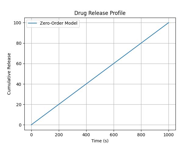
The Zero-Order model describes a constant rate of drug release over time. According to this model, the cumulative amount of drug released at time $t$ is given by:
$$ M_t = M_0 + k_0 t $$
where:
- $M_t (mg)$ is the cumulative absolute amount of drug released at time $t$.
- $M_0 (mg)$ is the initial amount of drug in the system. $M_0$ defaults to zero in this model.
- $k_0 (\frac{mg}{s})$ is the zero-order release rate constant.
Applications
- Tablets with extended release
- Transdermal Patches
- Implantable Device
- Intraocular Implants
- Infusion Systems
First-Order
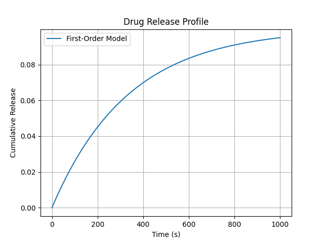
The first-order drug release model describes a process where the rate of drug release is proportional to the remaining amount of drug in the system. According to this model, the cumulative amount of drug released at time $t$ is given by:
$$ M_t = M_0 (1 - e^{-kt}) $$
where:
- $M_t (mg)$ is the cumulative absolute amount of drug released at time $t$.
- $M_0 (mg)$ is entire releasable amount of drug (the asymptotic maximum).
- $k (\frac{1}{s})$ is the first-order release rate constant.
Applications
- Immediate-release tablets and capsules
- Liquid drug formulations (oral solutions, intravenous injections)
- Controlled-release matrix systems
- Elastomeric infusion pumps
Higuchi
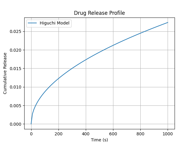
The Higuchi model describes the release of a drug from a matrix system, where the drug diffuses through a porous medium. The Higuchi equation addressed important aspects of drug transport and release from planar devices. According to this model, the cumulative amount of drug released at time $t$ is given by:
$$ M_t = \sqrt{D(2c_0 - c_s)c_st} $$
where:
- $M_t (\frac{mg}{cm^2})$ is the cumulative absolute amount of drug released at time $t$
- $D ({\frac{cm^2}{s}})$ is the drug diffusivity in the polymer carrier
- $c_0 (\frac{mg}{cm^3})$ is the initial drug concentration (total concentration of drug in the matrix)
- $c_s (\frac{mg}{cm^3})$ is the solubility of the drug in the polymer (carrier)
⚠️ The Higuchi model assumes that $c_0 \ge c_s$
Applications
- Matrix Tablets
- Hydrophilic polymer matrices
- Controlled - Release Microspheres
- Semisolid Systems
- Implantable Drug delivery systems
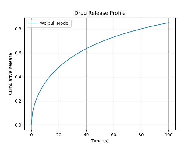
Weibull
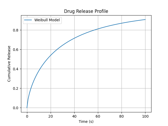
Weibull model is an empirical model used to describe drug release kinetics from various pharmaceutical dosage forms. It is characterized by a flexible empirical equation that captures various release kinetics. According to this model, the cumulative amount of drug released at time $t$ is given by:
$$ M_t = M \left(1 - e^{-at^b}\right) $$
where:
- $M_t (mg)$ is the cumulative absolute amount of drug released at time $t$
- $M (mg)$ is the total amount of drug released at infinite time
- $a$ is the scale parameter (related to the release rate)
- $b$ is the shape parameter (indicates the release mechanism)
Applications
- Controlled-release modeling
- Dissolution profiling
- Comparative studies
- Vivo predictions
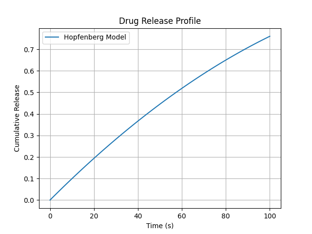
Hopfenberg
The Hopfenberg model describes drug release from surface-eroding polymers with a constant surface area. It is particularly useful for modeling drug release from biodegradable polymers where the drug is uniformly distributed throughout the matrix. According to this model, the cumulative amount of drug released at time $t$ is given by:
$$ M_t = M_{\infty} \left(1 - \left(1 - \frac{k_0t}{c_0 a_0}\right)^n\right) $$
where:
- $M_t (mg)$ is the cumulative absolute amount of drug released at time $t
- $M_{\infty} (mg)$ is the total amount of drug released at infinite time
- $k_0 (\frac{mg}{mm^2 s})$ is the surface erosion rate constant
- $c_0 (\frac{mg}{mm^3})$ is the initial drug concentration in the polymer matrix
- $a_0 (mm)$ is the initial radius (for spheres) or half-thickness (for slabs) of the device
- $n$ is the geometry-dependent exponent (1 for slabs, 2 for cylinders, 3 for spheres)
Applications
- Biodegradable Implants
- Surface-eroding drug delivery systems
- Transdermal Patches
- Injectable depots
Curve Fitting
The models above calculate a release profile from known parameters. The CurveFit class does the opposite operation. It calculates the parameters of a model from measured experimental data. CurveFit uses the non-linear least squares method. This method decreases the difference between the measured release and the calculated release.
CurveFit gives the quality of the fit as the coefficient of determination:
$$ R^2 = 1 - \frac{\sum_i \left(M_i - \hat{M}_i\right)^2}{\sum_i \left(M_i - \bar{M}\right)^2} $$
where:
- $M_i (mg)$ is the measured drug release at time $t_i$
- $\hat{M}_i (mg)$ is the drug release that the model calculates at time $t_i$
- $\bar{M} (mg)$ is the mean value of the measured drug release
An $R^2$ value near 1 shows a good fit. A low value shows that the model does not describe the data correctly.
You can fit all the models above. This table gives the name and the parameters of each model:
| Model Name | Parameters |
|---|---|
zero_order |
M0, k0 |
first_order |
M0, k |
higuchi |
D, c0, cs |
weibull |
M, a, b |
hopfenberg |
M, k0, c0, a0, n |
The fit method starts from a value of 1 for each unknown parameter, and keeps all the parameters positive. If the result is not good, give your own values in the initial_guess and bounds arguments. These arguments contain only the unknown parameters. The get_result method gives the result of the last fit again.
The fit method returns a FitResult object, where:
model_nameis the name of the fitted modelparametersis a dictionary of the known and the calculated parameter valuesr_squaredis the fit's coefficient of determinationmodelis a model object with the calculated parameters. You can simulate and plot this model.
Known Parameters
If you know the value of a parameter, give it in the known_parameters argument. Use the parameter names in the table above. CurveFit keeps these values constant and calculates only the other parameters.
⚠️ All the parameters of a model cannot always be calculated from a release profile. Some models use a group of parameters only as one product or one ratio. Many different combinations of these parameters give the same value for this group. Thus, the fit has no unique solution, and the calculated values can be different from the true physical values. To prevent this problem, give at least two parameters of each group in the known_parameters argument. Two of the models have such a group:
- The Higuchi model uses $D$, $c_0$ and $c_s$ only in the product $D(2c_0 - c_s)c_s$. Give two of these three parameters, for example
known_parameters={"c0": 1, "cs": 0.5}. - The Hopfenberg model uses $k_0$, $c_0$ and $a_0$ only in the ratio $\frac{k_0}{c_0 a_0}$. Give two of these three parameters, and also the geometry factor $n$, for example
known_parameters={"c0": 0.0374, "a0": 3.51, "n": 2}. Also, $n$ is always assumed to be known because the user should know the shape of the device.
Applications
- Analysis of dissolution test data
- Estimation of the release rate constants
- Selection of the correct model for an experiment
- Comparison of different formulations
- Quality control of production batches
Usage
Zero-Order Model
from drux import ZeroOrderModel
model = ZeroOrderModel(k0=0.1, M0=0)
model.simulate(duration=1000, time_step=10)
model.plot(show=True)
First-Order Model
from drux import FirstOrderModel
model = FirstOrderModel(k=0.003, M0=0.1)
model.simulate(duration=1000, time_step=10)
model.plot(show=True)
Higuchi Model
from drux import HiguchiModel
model = HiguchiModel(D=1e-6, c0=1, cs=0.5)
model.simulate(duration=1000, time_step=10)
model.plot(show=True)
Weibull Model
from drux import WeibullModel
model = WeibullModel(M=1, a=0.095, b=0.7)
model.simulate(duration=100, time_step=1)
model.plot(show=True)
Hopfenberg Model
from drux import HopfenbergModel
model = HopfenbergModel(M=1, k0=0.00067, c0=0.0374, a0=3.51, n=2)
model.simulate(duration=100, time_step=1)
model.plot(show=True)
Curve Fitting
from drux import CurveFit
time = [0, 10, 20, 30, 40, 50, 60, 70, 80, 90, 100]
release_profile = [0, 0.35, 0.48, 0.57, 0.63, 0.69, 0.73, 0.77, 0.80, 0.83, 0.85]
fitter = CurveFit(model_name="weibull", time=time, release_profile=release_profile)
result = fitter.fit()
print(result.parameters)
print(result.r_squared)
result.model.simulate(duration=100, time_step=1)
result.model.plot(show=True)
Issues & bug reports
Just fill an issue and describe it. We'll check it ASAP! or send an email to drux@openscilab.com.
- Please complete the issue template
You can also join our discord server

References
1- T. Higuchi, "Rate of release of medicaments from ointment bases containing drugs in suspension," Journal of Pharmaceutical Sciences, vol. 50, no. 10, pp. 874–875, 1961.
2- D. R. Paul, "Elaborations on the Higuchi model for drug delivery," International Journal of Pharmaceutics, vol. 418, no. 1, pp. 13–17, 2011.
3- R. T. Medarametla, K. V. Gopaiah, J. N. Suresh Kumar, G. Anand Babu, M. Shaggir, G. Raghavendra, D. Naveen Reddy, and B. Venkamma, "Drug Release Kinetics and Mathematical Models," International Journal of Science and Research Methodology, vol. 27, no. 9, pp. 12–19, Sep. 2024.
4- R. Vaju and K. V. Murthy, "Development and validation of new discriminative dissolution method for carvedilol tablets," Indian Journal of Pharmaceutical Sciences, vol. 73, no. 5, pp. 527–536, Sep. 2011.
5- S. Dash, "Kinetic modeling on drug release from controlled drug delivery systems," Acta Poloniae Pharmaceutica, 2010.
6- K. H. Ramteke, P. A. Dighe, A. R. Kharat, S. V. Patil, Mathematical models of drug dissolution: A review, Sch. Acad. J. Pharm., vol. 3, no. 5, pp. 388-396, 2014.
7- C. Corsaro, G. Neri, A. M. Mezzasalma, and E. Fazio, "Weibull modeling of controlled drug release from Ag-PMA nanosystems," Polymers, vol. 13, no. 17, p. 2897, 2021.
8- H. B. Hopfenberg, "Controlled release from erodible slabs, cylinders, and spheres," in Controlled Release Polymeric Formulations, ACS Symposium Series, vol. 33, pp. 26–32, 1976.
9- H. V. Chavda, M. S. Patel, and C. N. Patel, "Preparation and in vitro evaluation of guar gum based triple-layer matrix tablet of diclofenac sodium," Research in Pharmaceutical Sciences, vol. 7, no. 1, pp. 57–64, Jan. 2012.
Show your support
Star this repo
Give a ⭐️ if this project helped you!
Donate to our project
If you do like our project and we hope that you do, can you please support us? Our project is not and is never going to be working for profit. We need the money just so we can continue doing what we do ;-) .

Changelog
All notable changes to this project will be documented in this file.
The format is based on Keep a Changelog and this project adheres to Semantic Versioning.
Unreleased
0.5 - 2026-10-14
Added
CurveFitclassCurveFitclass documentationFitResultclass
Changed
_model_functionmethod refactored_model_functionmethod renamed tomodel_function- Dependencies structure modified
0.4 - 2026-05-18
Added
- Hopfenberg model
0.3 - 2025-12-08
Added
- Weibull model
- Logo
__repr__method for models
Changed
Python 3.14added totest.yml
0.2 - 2025-09-27
Added
- Zero-order model
- First-order model
Changed
README.mdmodified- Test system modified
- Release range bug in
time_for_releasefixed matplotlibimport bug fixedplotmethod modified
0.1 - 2025-07-27
Added
- Base model
- Higuchi model
2 maintainers


Metadata
2 maintainers
Release files for drux 0.5
For a detailed explanation of source distributions (sdists) and built distributions (wheels), please see the package formats documentation.
Source distribution (sdist)
| File | Size | Uploaded | |
|---|---|---|---|
| drux-0.5.tar.gz | 28.7 kB | Details |
Built distribution (wheel)
| File | Interpreter | ABI | Platform | Reset |
|---|---|---|---|---|
| drux-0.5-py3-none-any.whl | Python 3 | none | any | Details |
Total release size: 49.3 kB
Release files / drux-0.5.tar.gz
| Download URL | drux-0.5.tar.gz |
|---|---|
| Size | 28.7 kB |
| Tags | Source |
|
SHA-256 checksum How to use checksums |
a41723d46bf8d763b8b0bd03ebb64b5994edc75568d668455bf7c724ced9897a
|
|
BLAKE2b-256 checksum How to use checksums |
cdd72d17421c16230e6673b69779a17965e029a1a2787ac57a34dcef07ac5a14
|
| Upload date | |
|
Uploaded using Trusted Publishing? What is trusted publishing? |
No |
| Uploaded via |
twine/7.0.0 CPython/3.14.8
|
Release files / drux-0.5-py3-none-any.whl
| Download URL | drux-0.5-py3-none-any.whl |
|---|---|
| Size | 20.7 kB |
| Tags | Python 3 |
|
SHA-256 checksum How to use checksums |
ebde210504bcda970f6a8894ecfaac578905ccd5dce391386a307a2d86d5e84c
|
|
BLAKE2b-256 checksum How to use checksums |
29f8e5713be71c977ac86762ec7bdbe3398ed6ad35a2faacc1dd7016a4f2cde5
|
| Upload date | |
|
Uploaded using Trusted Publishing? What is trusted publishing? |
No |
| Uploaded via |
twine/7.0.0 CPython/3.14.8
|














