
DWDPheno
Plant-phenology observations of the German Weather Service (DWD), as tidy pandas tables





Install · Quick start · Stations · Crops · Output · Quality · Comparing · BBCH series · CLI · Desktop app · Data & licences
dwdpheno downloads the phenological observations of the
DWD Climate Data Center:
more than a century of dates at which sowing, emergence, flowering, ripening and harvest were
observed for arable crops, fruit, vines and wild plants at several thousand stations across
Germany.
DWD publishes this as hundreds of fixed-width text files spread over reporter types, plant
groups and historical/recent folders, some in several overlapping versions, with station metadata,
phase definitions and BBCH codes in separate files. dwdpheno handles all of that:
- finds the files for the crops you name (English or German), using only the newest version of each historical file;
- selects stations by id, name, federal state, county, city, radius, nearest k, bounding box or polygon. Every station gets its county (BKG VG2500) and nearest place;
- returns one tidy table with station metadata, English (plus German and Latin) plant names, English phase names, BBCH codes and decoded quality flags, with historical/recent duplicates removed;
- builds BBCH time series: crop cycles are detected from the data and drawn as a shape-preserving PCHIP curve, with day-of-year statistics and trends on top;
- caches everything on disk, so repeated runs are fast and can work offline.
It depends only on pandas and numpy (matplotlib is optional, for plots) and uses the
standard library for HTTP.
Prefer clicking to coding? DWDPheno Studio is a desktop app for Windows and Linux with a map of Germany, station selection, downloads and BBCH plots. Installers are on the releases page.
Installation
pip install dwdpheno            # core
pip install "dwdpheno[plot]"    # + matplotlib for plot_station()
Python 3.9 or newer, pandas 1.5 to 3.x.
Quick start
import dwdpheno as dp

# winter wheat at all stations in the rural district (Landkreis) of Kassel, 2015-2024
obs = dp.download("winter wheat", years=(2015, 2024), county="Kassel rural district")

nk = obs.query("station_name == 'Niederkaufungen' and reporter == 'annual'")
nk[["station_name", "crop", "phase_name", "bbch_code", "date", "day_of_year"]].head(4)
#    station_name         crop                phase_name bbch_code       date  day_of_year
# Niederkaufungen winter wheat     beginning of shooting        31 2015-05-07          127
# Niederkaufungen winter wheat      beginning of heading        51 2015-06-03          154
# Niederkaufungen winter wheat beginning of mil ripeness        75 2015-07-08          189
# Niederkaufungen winter wheat           yellow ripeness        87 2015-07-19          200

stats  = dp.summary(obs)                  # mean / sd / trend of day of year per phase
curves = dp.series(obs)                   # BBCH points + smooth curve per season
dp.plot_station(obs, station_id=9646)     # needs matplotlib

obs.to_csv("wheat_kassel.csv", index=False)
From the shell:
dwdpheno download --crops "winter wheat" --years 2015-2024 --county "Kassel rural district" --out wheat.csv
Selecting stations
dp.stations(**selection) returns the station table; dp.download(crops, **selection) takes
the same keywords. All criteria you give are combined with AND.
| keyword | CLI | meaning |
|---|---|---|
station_id= |
--station-id 1,2 |
exact ids (int, list or "1,2") |
name= |
--name Kassel |
station-name match; a comma or a list means OR |
state= |
--state Hessen |
federal state (Bundesland) |
county= |
--county "Kassel rural district" |
county, matched against "{county} {county_type} {county_type_de}", so "Landkreis Kassel" works too |
city= |
--city Göttingen |
centre = best-matching place (exact name first, then largest population) |
lat=, lon= |
--lat 51.3 --lon 9.5 |
centre point |
radius_km= |
--radius 25 |
km around the centre (default 25 when a centre is given) |
nearest= |
--nearest 5 |
the k closest stations to the centre (instead of a radius) |
bbox=(s, w, n, e) |
--bbox s,w,n,e |
latitude/longitude box |
polygon=[(lat, lon), ...] |
--polygon "lat lon;lat lon;..." |
point in polygon (even-odd rule) |
reporter= |
--reporter annual|immediate|both |
DWD reporter network (default both) |
active=True |
--active |
only stations that are still active |
dp.stations(station_id=[9646, 9768])
dp.stations(name="Kaufungen")                       # Niederkaufungen, Oberkaufungen
dp.stations(name="Gießen, Marburg")                 # OR
dp.stations(state="Hessen", active=True)
dp.stations(county="Kassel rural district")         # the rural district only
dp.stations(county="Landkreis Kassel")              # the same, with the German type
dp.stations(county="Kassel")                        # the rural district and the city of Kassel
dp.stations(city="Göttingen", radius_km=30)         # adds distance_km, sorted by distance
dp.stations(lat=51.31, lon=9.49, nearest=5)
dp.stations(bbox=(51.0, 9.0, 51.6, 10.0))
dp.stations(polygon=[(51.0, 9.2), (51.4, 9.2), (51.4, 9.8), (51.0, 9.8)])
dp.stations(reporter="immediate")
Only stations that have data. Add crops= (and optionally years=, partition=,
quality=, quality_level=) and you get only the selected stations that actually observed
those crops, with the number of observations and their year range. The counts are exactly what
download() would return with the same arguments (the data files are downloaded to count them).
For example, the stations that observed winter wheat in Hessen since 2015:
st = dp.stations(state="Hessen", crops="winter wheat", years=(2015, 2024))
len(st)                                    # 103 (of 577 stations in Hessen)
st.sort_values("n_observations", ascending=False)[
    ["station_id", "station_name", "county", "n_observations", "first_year", "last_year"]].head(3)
#  station_id              station_name         county  n_observations  first_year  last_year
#        9646           Niederkaufungen         Kassel             130        2015       2024
#       14140  Friedberg-Bruchenbrücken  Wetteraukreis             130        2015       2024
#        9593             Margretenhaun          Fulda             129        2015       2024
dwdpheno stations --state Hessen --crops "winter wheat" --years 2015-2024 --out wheat_stations.csv
Text matching ignores case, umlauts and punctuation: ä→ae ö→oe ü→ue ß→ss, accents are
removed, - _ . , ( ) count as blanks, and a query matches when each of its words appears in the
text. So "Landkreis Kassel" matches the county text "Kassel rural district Landkreis",
"goettingen" matches "Göttingen", and "Kassel" matches both Kassel counties.
Station table columns
| column | meaning |
|---|---|
station_id |
DWD station id (int) |
station_name |
|
latitude, longitude, elevation_m |
WGS84 degrees (4 decimals, as published), metres (integer) |
state |
federal state as published by DWD |
county, county_type, county_id |
county (Kreis) from BKG VG2500 point-in-polygon; county_type is rural district (Landkreis), district (Kreis) or urban district (Kreisfreie Stadt, Stadtkreis); county_id = AGS key, e.g. 06633; empty outside |
nearest_place, nearest_place_km |
nearest town/village (GeoNames, population ≥ 1000), km with 2 decimals |
naturraumgruppe, naturraum |
natural region (group) |
active_until |
dissolution date dd.mm.yyyy; empty = still active |
reporter |
annual, immediate or both |
distance_km |
only when the selection has a centre point (2 decimals) |
n_observations, first_year, last_year |
only with crops=: observations of those crops at the station (after the year, partition, reporter and quality filters and the historical/recent de-duplication) and their year range |
Places can be searched directly: dp.places("Frankfurt") returns name, latitude, longitude,
population, state.
Crops and species
Crop, plant and phase names come from DWD's own reference tables
(PH_Beschreibung_Pflanze.txt
for English, German and Latin plant names,
PH_Beschreibung_Phase.txt
for English phase names). Every DWD file token (Winterweizen, Apfel_fruehe_Reife, …) is
matched to its plant, which gives this catalog:
dp.crops()
#                   crop            crop_de            species  objekt_id           dwd_token  group         reporters  first_year  last_year  files
#                   beet              Rüben      Beta vulgaris         25               Ruebe  crops  annual;immediate        <NA>       2026      3
#           spring wheat       Sommerweizen  Triticum aestivum        206        Sommerweizen  crops            annual        1927       1990      1
#           winter wheat       Winterweizen  Triticum aestivum        202        Winterweizen  crops  annual;immediate        1925       2026      4
#                  apple              Apfel    Malus domestica        310               Apfel  fruit  annual;immediate        1925       2026      4
# apple (early ripeness) Apfel, frühe Reife    Malus domestica        311  Apfel_fruehe_Reife  fruit            annual        1929       2026      2
# ...                                                                  (77 crops, sorted by group and English name)
first_year/last_year come from the historical file names; when a crop also has a recent
file, last_year is the current year (a few files carry no years at all). group is one of
crops wild fruit vine farming.
Naming crops. You can use the English name, the German name or the DWD token, in any case and with or without umlauts:
- a name that equals a crop's English name, German name or token selects exactly that crop:
"apple"gives only apple,"Apfel_fruehe_Reife"only apple (early ripeness); - otherwise every word you give must be the start of a word of one of the names:
"wheat"gives winter wheat and spring wheat,"app"all three apples,"lime"both lime trees, and"apple early"the early-ripening apples."ash"gives ash but not rowan (Eberesche).
dp.download("winter wheat", ...)            # one crop
dp.download(["winter barley", "maize"], ...)
dp.download("Apfel", ...)                   # German name
dp.download("wheat", ...)                   # winter + spring wheat
In the downloaded data, crop / crop_de / species are the English / German / Latin names of
each row's plant (objekt_id).
Phases and BBCH codes
dp.phases("winter wheat")
# objekt_id          crop  phase_id                            phase_name bbch_code
#       202  winter wheat        10  beginning of tilling sowing drilling         0
#       202  winter wheat        12                beginning of emergence        10
#       202  winter wheat        15                 beginning of shooting        31
#       ...
#       202  winter wheat        24                               harvest      <NA>

dp.find_bbch(5)                  # every plant that uses phase_id 5
dp.bbch_for(18, objekt_id=202)   # '51' (winter wheat, beginning of heading)
Phase names are DWD's English phase names. BBCH codes come from the phase definitions of each
plant group; phases without a BBCH code (e.g. harvest) have an empty bbch_code.
Years
years takes 2005, an inclusive range (2000, 2020), a list [1990, 1995, 2000], or
None for everything (the CLI uses 2005, 2000-2020 or 1990,1995). It filters on DWD's
reference year (Referenzjahr). For winter crops that is the harvest year, and the autumn
sowing of the next crop falls in the same reference year (see
BBCH time series).
Output columns
dp.download() returns one row per observation, sorted by crop, station_id, year, date, phase_id.
Everything is in English except the proper names of places (stations, states, counties, natural
regions).
| column | meaning |
|---|---|
station_id, station_name, latitude, longitude, elevation_m, state, county |
station metadata |
crop, crop_de, species |
English, German and Latin name of the row's plant, e.g. winter wheat, Winterweizen, Triticum aestivum |
objekt_id |
DWD plant id |
phase_id, phase_name |
phenological phase (English name from DWD, e.g. beginning of heading) |
bbch_code |
BBCH code as text ("31"); empty when DWD defines none |
year |
DWD's reference year (Referenzjahr; the harvest year) |
date |
date of the observation (datetime64; ISO YYYY-MM-DD in files) |
day_of_year |
day of year as published by DWD (Jultag) |
quality_byte, quality_byte_meaning |
1 not flagged, 2 corrected, 3 confirmed despite flag, 5 doubtful, 8 incorrect, 0 no quality byte |
quality_level, quality_level_meaning |
1 pre-load check only, 2 pre-load check (immediate reporters), 7 ROUTKLI checked, 10 ROUTKLI checked + corrected |
reporter |
annual (Jahresmelder) or immediate (Sofortmelder) |
partition |
historical or recent |
source_file |
DWD file the row came from |
Where the historical and recent files overlap, rows are de-duplicated on
(station_id, objekt_id, phase_id, year, reporter) and the recent row is kept.
Other options: partition="historical" | "recent" | "both", reporter=...,
quality= / quality_level= (see Data quality; default: keep everything),
verbose=True (progress on stderr) and progress=callback(i, n, text).
Data quality
Every DWD observation carries two quality flags, and dwdpheno keeps both:
quality byte (quality_byte) |
meaning | quality level (quality_level) |
meaning | |
|---|---|---|---|---|
1 |
not flagged | 1 |
pre-load check only | |
2 |
corrected | 2 |
pre-load check (immediate reporters) | |
3 |
confirmed despite flag | 7 |
ROUTKLI checked | |
5 |
doubtful | 10 |
ROUTKLI checked + corrected | |
8 |
incorrect | |||
0 |
no quality byte (a missing byte counts as 0) |
By default nothing is filtered: every observation is returned, and its quality is shown in
the download columns, in the series point rows, in the summary counts and in the plot. To
keep only some codes, pass quality= (quality bytes) and/or quality_level= (quality levels)
to download, series, summary or plot_station, or --quality / --quality-level on the
command line:
obs   = dp.download("winter wheat", years=(2015, 2024), county="Kassel rural district")
clean = dp.download("winter wheat", years=(2015, 2024), county="Kassel rural district",
                    quality=[1, 2, 3])            # drop doubtful (5), incorrect (8), no byte (0)
dp.download("winter wheat", county="Kassel rural district", quality_level=[7, 10])  # checked only

dp.series(obs, quality=[1, 2, 3])                  # same options on an existing table
dp.summary(obs, quality=[1, 2, 3])
dp.plot_station(obs, 9768, quality=[1, 2, 3])
dwdpheno download --crops "winter wheat" --county "Kassel rural district" --quality 1,2,3 --out clean.csv
dwdpheno summary --in wheat.csv --quality-level 7,10 --out summary.csv
In the downloaded table the historical/recent de-duplication happens first and the quality
filter afterwards, so a filtered-out recent row never lets an older historical copy back in.
summary() reports how many observations of each phase had which flag; at Bad
Emstal-Merxhausen (9768) two doubtful early "beginning of shooting" dates noticeably change the
trend:
dp.summary(obs).query("station_id == 9768 and phase_id == 15")
#  n  mean_doy  sd_doy  trend_days_per_decade  n_not_flagged  n_corrected  n_confirmed  n_doubtful  n_incorrect  n_no_quality_byte  quality_levels
# 15     95.27    6.72                  -6.08             11            1            1           2            0                  0            7;10
dp.summary(obs, quality=[1, 2, 3]).query("station_id == 9768 and phase_id == 15")
# 13     96.92    5.33                  -1.21             11            1            1           0            0                  0            7;10
BBCH time series and plots
DWD's reference year (Referenzjahr) is not a crop cycle. For winter wheat, year 2024 holds the April–July 2024
stages and also the October 2024 sowing of the next crop. dp.series() therefore finds the
cycles in the data:
- per station and crop, take the observations with a numeric BBCH code (all of them, unless
you pass
quality=/quality_level=) and sort them by date; - start a new cycle when BBCH drops by more than 20 below the cycle's maximum (harvest → sowing) or when more than 300 days pass between two observations;
seasonis the calendar year of the cycle's last observation, i.e. the harvest year. A cycle that is not finished yet (sown in autumn, no spring data yet) would get the same year as the cycle before it; it gets the previous season + 1 instead;- inside each cycle BBCH is interpolated over time with the monotone piecewise-cubic Hermite interpolant (PCHIP, Fritsch–Carlson). It keeps the shape of the data and does not overshoot.
s = dp.series(obs, station_id=9646, crops="winter wheat", step_days=1)
#  kind  station_id          crop  season        date        t  season_doy   bbch  phase_id                            phase_name  quality_byte  quality_byte_meaning  quality_level        quality_level_meaning
# point        9646  winter wheat    2024  2023-10-03  19633.0      -89.00   0.00        10  beginning of tilling sowing drilling             1           not flagged             10  ROUTKLI checked + corrected
# point        9646  winter wheat    2024  2023-10-03  19633.0      -89.00   0.00        10  beginning of tilling sowing drilling             1           not flagged              7              ROUTKLI checked
#   ...
# curve        9646  winter wheat    2024  2023-10-04  19634.0      -88.00   0.84      <NA>                                  <NA>          <NA>                  <NA>           <NA>                         <NA>
kind is point (an observation) or curve (a sample every step_days from the first to the
last observation of the cycle, both ends included). t is days since 1970-01-01 and
season_doy the day of the season (1 = 1 January of the harvest year, negative = the autumn
before); t, season_doy and bbch are rounded to 2 decimals. station_id and crops take
lists. Point rows carry the observation's quality flags; curve rows
leave the phase and quality columns empty.
import dwdpheno as dp

obs = dp.download(["winter wheat", "winter barley", "maize"], years=(2015, 2024),
                  county="Kassel rural district")
ax = dp.plot_station(obs, station_id=9768, years=(2020, 2023))
ax.figure.savefig("bbch_series.png", dpi=150)
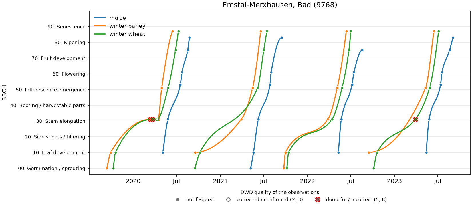
plot_station(obs, station_id, crops=None, ax=None, years=None, quality=None, quality_level=None)
draws real dates on the x axis, the BBCH principal growth stages (0–90) on the y axis, and one
colour per crop, with the observations as points and a smooth curve per crop cycle. The markers
show the DWD quality: filled dots are not flagged (or have no quality byte), hollow circles are
corrected or confirmed despite a flag, and crosses with a red edge are doubtful or incorrect
(above: early "beginning of shooting" reports in March 2020 and March 2023). Pass ax= to draw
into your own figure.
Comparing stations, crops and seasons
dp.plot_series() draws any number of stations, crops and seasons together. Pick the x axis,
what the colours stand for, and optionally one panel per station or crop:
| argument | values | |
|---|---|---|
station_id, crops, years |
one or several (default: everything in obs) |
what to draw |
x |
"date" (real dates) or "season_doy" |
season_doy puts every season on one axis: day 1 = 1 January of the harvest year, negative = the autumn before |
color_by |
"crop", "station" or "season" |
one colour per value |
facet |
None, "station" or "crop" |
small multiples with shared axes |
When a second key also varies (e.g. several crops while colouring by station), it gets its own
line styles and legend. The quality markers are the same as in plot_station(), which is now a
shorthand for plot_series(obs, station_id, x="date", color_by="crop").
Winter wheat in season 2023 at four stations from the Baltic coast to Bavaria:
obs = dp.download("winter wheat", years=(2022, 2023), reporter="annual")
ax = dp.plot_series(obs, station_id=[12522, 7857, 9389, 10953], years=2023,
                    x="season_doy", color_by="station")
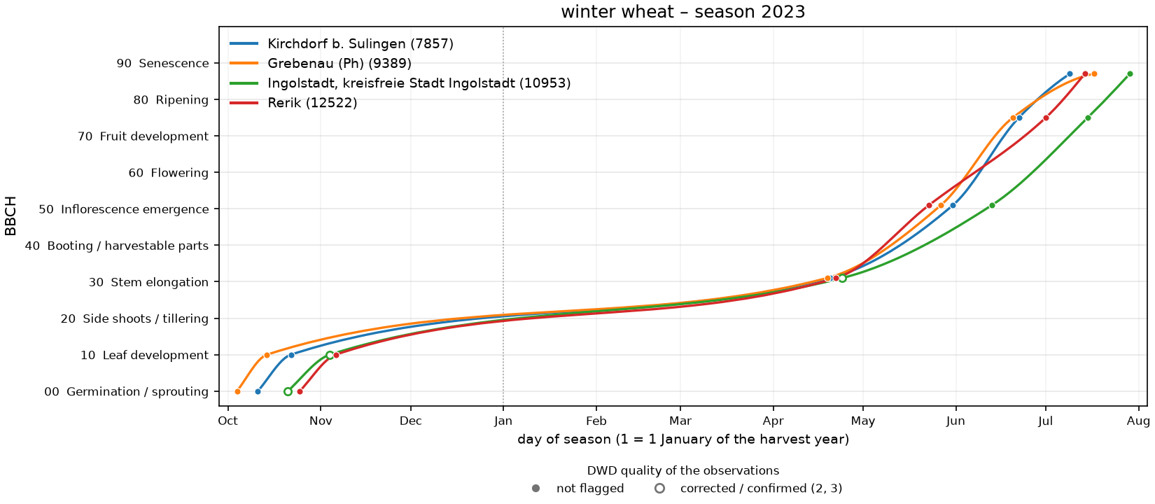
All four reached stem elongation (BBCH 31) within five days of each other (days 109–114, around 20 April), but Ingolstadt headed 13–21 days later than the others (day 164 against 143–151) and reached yellow ripeness on day 210 against 190–198.
Other combinations:
dp.plot_series(obs, station_id=9389, x="season_doy", color_by="season")   # one station, seasons overlaid
dp.plot_series(obs, station_id=[12522, 10953], x="season_doy",
               color_by="season", facet="station")                        # one panel per station

three = dp.download(["winter wheat", "winter barley", "maize"], years=(2021, 2023), station_id=9768)
dp.plot_series(three, x="season_doy", color_by="crop")                     # crops; seasons as line styles
series() gives the same day-of-season values in its season_doy column, for your own plots.
Phase dates over the years
dp.plot_phase_trend() plots the day of year of phenological phases against the year, with an
OLS trend line per phase and the trend in days per decade in the legend. Phases are given by id
or English name ("heading" finds beginning of heading); several stations are pooled per crop
and phase. For a single station the trends are the same as summary()'s trend_days_per_decade.
long = dp.download("winter wheat", years=(1991, 2024), station_id=9646, reporter="annual")
ax = dp.plot_phase_trend(long, phases=["beginning of shooting", "beginning of heading",
                                       "yellow ripeness", "harvest"])
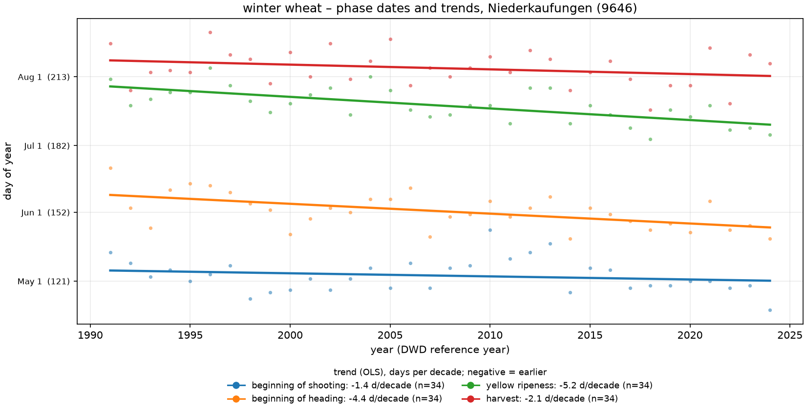
At Niederkaufungen, heading has moved 4.4 days per decade earlier since 1991 and yellow ripeness 5.2 days per decade, while shooting changed little (1.4 days per decade).
Summary statistics
dp.summary(obs)
# station_id          crop  objekt_id  phase_id             phase_name  bbch_code   n  first_year  last_year  mean_doy  sd_doy  min_doy  max_doy  trend_days_per_decade
#       9646  winter wheat        202        15  beginning of shooting         31  20        2015       2024    119.45    5.03      108      127                 -13.00
One row per (station_id, crop, objekt_id, phase_id) with the number of observations, the year
range and the mean, sample standard deviation, minimum and maximum day of year.
trend_days_per_decade is the OLS slope of day of year on year × 10, left empty when n < 3.
Mean, standard deviation and trend are rounded to 2 decimals. The last columns count the
observations per quality byte (n_not_flagged, n_corrected, n_confirmed, n_doubtful,
n_incorrect, n_no_quality_byte) and list the quality levels found (quality_levels, e.g.
7;10); summary(obs, quality=..., quality_level=...) filters first.
Command line
The dwdpheno command (also available as python -m dwdpheno) covers the same functions:
dwdpheno stations  [selection] [--crops A,B [--years ...] [--partition ...] [quality]]
                   [--format csv|json] [--out FILE]
dwdpheno crops     [--format csv|json] [--out FILE]
dwdpheno phases    [--crops A,B] [--format csv|json] [--out FILE]
dwdpheno download  --crops A,B [--years 2000-2020|2005|1990,1995] [selection] [quality]
                   [--partition historical|recent|both] [--format csv|json] [--out FILE]
dwdpheno series    --in OBS.csv [--station-id N] [--crops A] [--step-days 1] [quality] [--format csv|json] [--out FILE]
dwdpheno summary   --in OBS.csv [quality] [--format csv|json] [--out FILE]
dwdpheno places    --q NAME [--limit N] [--format csv|json] [--out FILE]
dwdpheno plot      --in OBS.csv [--station-id N,M] [--crops A,B] [--years 2019-2024]
                   [--x date|season_doy] [--color-by crop|station|season] [--facet station|crop]
                   [quality] --out FILE.png
dwdpheno plot-trend --in OBS.csv [--phases ID|NAME,...] [--station-id N,M] [--crops A] [--years ...]
                   [quality] --out FILE.png
dwdpheno version

selection:  --station-id --name --state --county --city --lat --lon --radius --nearest
            --bbox --polygon --reporter --active
quality:    --quality 1,2,3  --quality-level 7,10      (default: keep everything)
global:     --cache DIR|off  --offline  --quiet  --max-age-days 1  --data DIR
dwdpheno stations --city Göttingen --radius 20
dwdpheno stations --state Hessen --crops "winter wheat" --years 2015-2024
dwdpheno crops --format json --out crops.json
dwdpheno download --crops apple,pear --years 1990-2024 --state Sachsen --active --out fruit.csv
dwdpheno series --in fruit.csv --station-id 12345 --step-days 7 --out series.csv
dwdpheno summary --in fruit.csv --quality 1,2,3 --out summary.csv
dwdpheno plot --in fruit.csv --station-id 12345 --years 2015-2024 --out station.png
dwdpheno plot --in fruit.csv --station-id 12345,23456 --x season_doy --color-by station --years 2020 --out compare.png
dwdpheno plot-trend --in fruit.csv --phases "beginning of flowering" --out flowering_trend.png
- Without
--out, results go to stdout. CSV is comma-separated UTF-8 with empty cells for missing values. JSON is an array of objects withnullfor missing values. - Progress goes to stderr as
PROGRESS <i> <n> <text>(turn it off with--quiet); errors go to stderr asERROR <text>. - Exit codes:
0ok,1usage error,2no match,3network or I/O error.
Caching and offline use
Every downloaded file is kept in a local cache:
| platform | default location |
|---|---|
| Windows | %LOCALAPPDATA%\dwdpheno\cache |
| Linux / macOS | $XDG_CACHE_HOME/dwdpheno, else ~/.cache/dwdpheno |
or wherever the DWDPHENO_CACHE environment variable points. dp.default_cache_dir() shows
the path in use.
- Historical data files (
*_hist.txt) never change and are never downloaded again. - Directory listings, station metadata, phase definitions and recent files are refreshed after
max_age_days(default 1). offline=True(--offline) uses only what is already cached.cache=False(--cache off) turns the cache off, andcache="path"uses another folder.- If a refresh fails because of a network problem, the stale copy is used and a warning is issued.
Every function that talks to DWD (stations, crops, phases, download) accepts cache=,
offline= and max_age_days=.
Large crops come in large historical files (winter wheat is about 140 MB), because DWD publishes one file per crop for all stations. The first download takes a while; after that, selections run from the cache in seconds.
DWDPheno Studio — desktop app
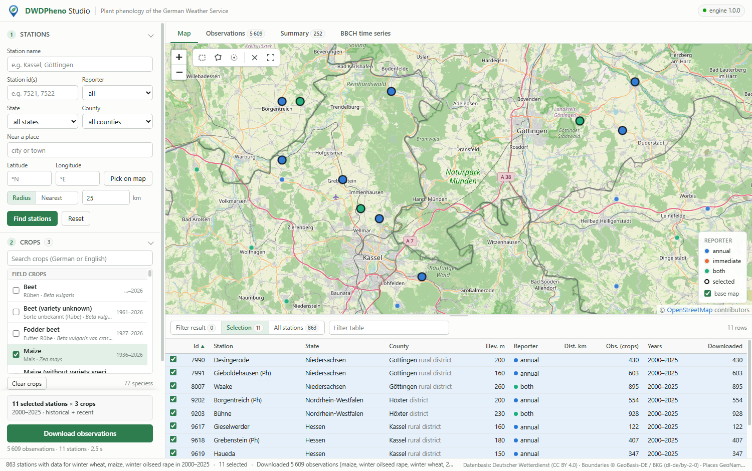
DWDPheno Studio is a desktop application for the same data, for people who'd rather click than code. Its engine is native Fortran, and it shows the data on a map and in charts. Everything in it is in English except the local names of stations and places.
- Map of Germany with every active DWD phenology station, state and county outlines, and an OpenStreetMap base map. Pick stations by clicking, with a box or lasso, by name or id, by state or county, around a place or coordinate (radius or nearest k).
- Only stations with data: as soon as you choose crops and years, the map, the tables and the selection tools show only the stations that observed those crops in those years, with the number of observations and the year range.
- 77 crops and wild plants with their English, German and Latin names, years and partitions, and one-click download with progress and cancel.
- Data quality: every DWD quality byte and quality level can be switched on or off. By default nothing is filtered, and the quality is shown in the observation table, the summary and on every plotted point.
- BBCH time series: the observed stages on their true dates, joined per season by a smooth, monotone PCHIP curve. Several stations, crops and seasons can be overlaid or shown as small multiples, on calendar dates or on a common day-of-season axis.
- Phase timing: the day of year of any phase against year, with OLS trend lines in days per decade.
- Summary table with day-of-year statistics and trends per station, crop and phase, and CSV, PNG and SVG export of every table and figure.
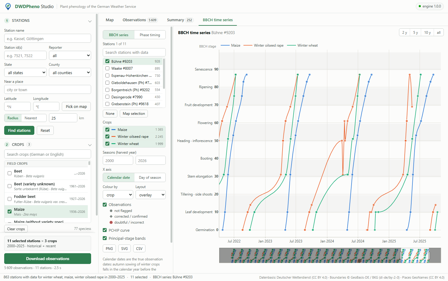 |
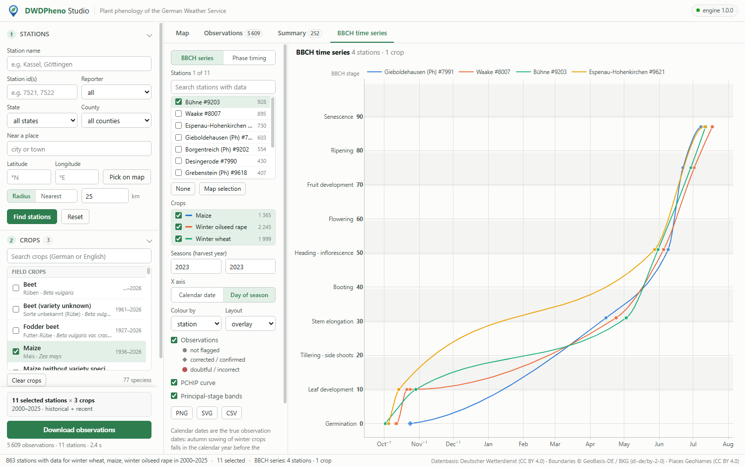 |
| BBCH stages on their true dates with the PCHIP curve per season | Four stations compared on the day-of-season axis |
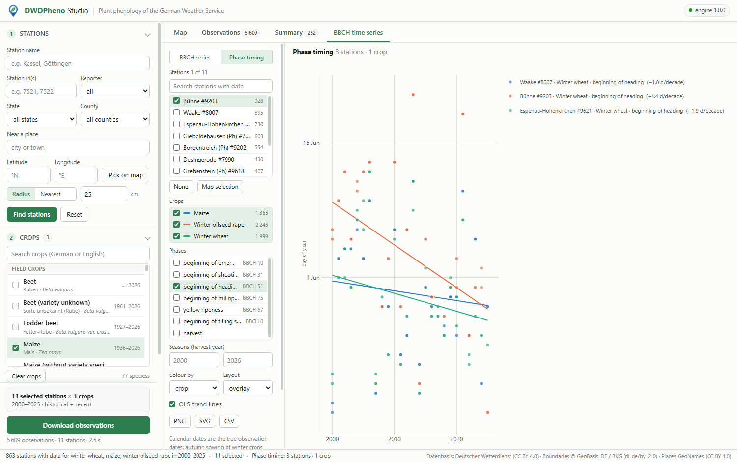 |
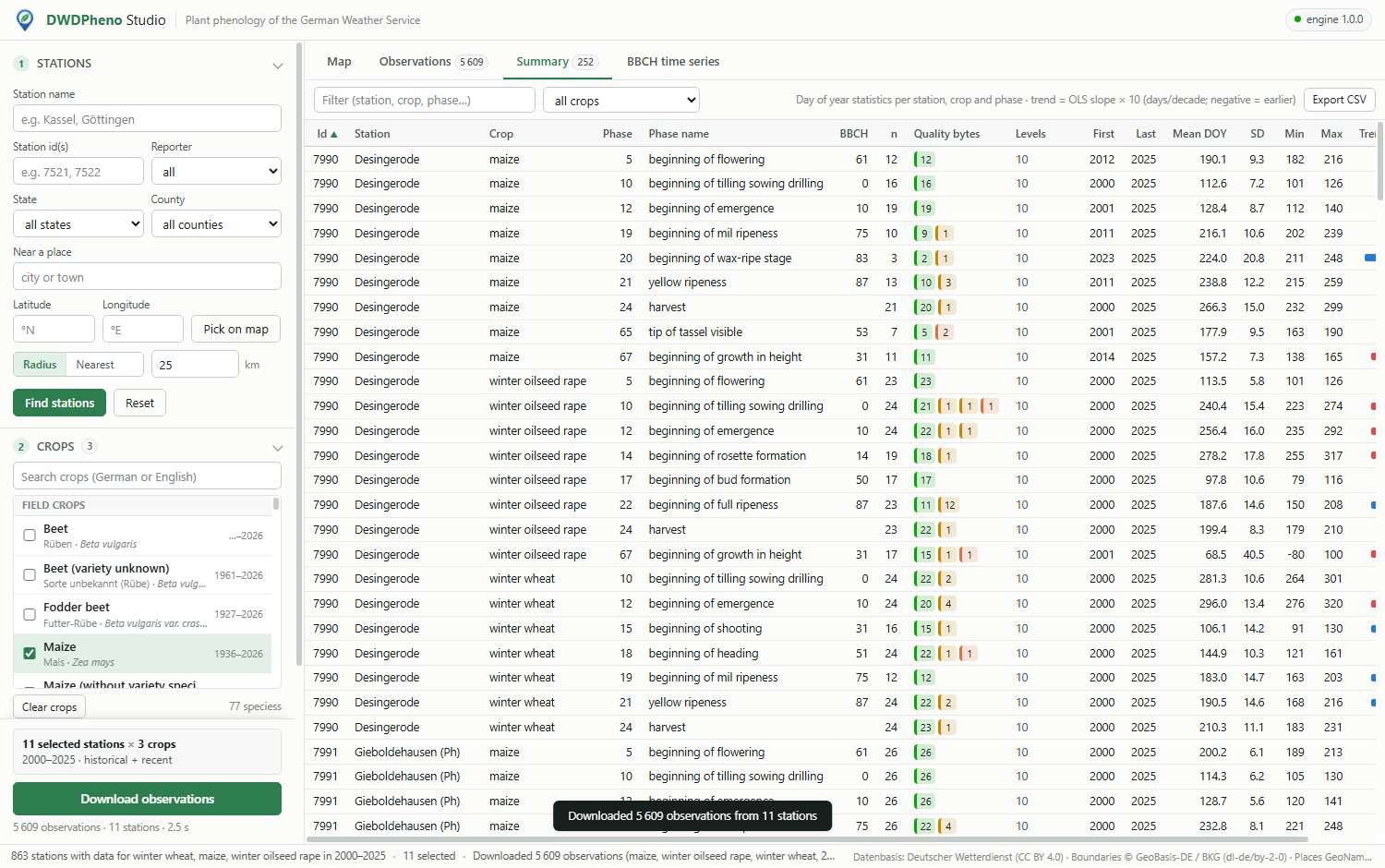 |
| Heading dates per year and trend for three stations | Summary statistics with the quality of the observations |
Download and install
Installers are attached to every GitHub release. No Python is needed: the engine is Fortran and the application is .NET with a web view, and everything it needs is inside the installer.
| Platform | File | How to install |
|---|---|---|
| Windows 10 / 11 (x64) | DWDPheno-Studio-1.0.0-setup.exe |
Run it. It installs for the current user without administrator rights (or for all users, if you choose). It uses the Microsoft Edge WebView2 runtime, which comes with Windows 11 and is installed automatically when missing. |
| Linux (x64, any distribution) | DWDPheno-Studio-1.0.0-linux-x64.run |
chmod +x DWDPheno-Studio-1.0.0-linux-x64.run && ./DWDPheno-Studio-1.0.0-linux-x64.run installs into ~/.local (run it with sudo to install into /opt for all users; --uninstall removes it). |
| Debian / Ubuntu | dwdpheno-studio_1.0.0_amd64.deb |
sudo apt install ./dwdpheno-studio_1.0.0_amd64.deb |
| Linux (manual) | dwdpheno-studio-1.0.0-linux-x64.tar.gz |
tar xf dwdpheno-studio-1.0.0-linux-x64.tar.gz && cd dwdpheno-studio-1.0.0 && ./install.sh |
On Linux, start DWDPheno Studio from the application menu or run dwdpheno-studio. It opens in
your web browser at http://127.0.0.1:8060 (the server listens on this computer only). The Linux
build needs the system packages libgfortran5 and curl. The .deb installs them, and the .run
installer does so when run with sudo.
Downloaded DWD files are cached in %LOCALAPPDATA%\DWDPheno\cache (Windows) or
~/.local/share/DWDPheno/cache (Linux). Historical files are kept for good, and listings and recent
files are refreshed daily.
DWDPheno Studio is free for scientific, educational and personal use. It is distributed as installers only, and its licence is shown during installation. The Python package in this repository is MIT-licensed open source.
Data sources and licences
- Phenological observations, station metadata, phase definitions: Deutscher Wetterdienst (DWD), Climate Data Center, https://opendata.dwd.de/climate_environment/CDC/observations_germany/phenology/. Licence CC BY 4.0. When you publish results, credit the source: "Datenbasis: Deutscher Wetterdienst" (data basis: German Weather Service), and mention any changes you made.
- Administrative boundaries (states and districts, bundled in
dwdpheno/data/): © GeoBasis-DE / BKG, VG2500, Datenlizenz Deutschland – Namensnennung – Version 2.0 (dl-de/by-2-0). - Places (bundled in
dwdpheno/data/cities.txt): GeoNames, CC BY 4.0.
The bundled reference data can be rebuilt with python tools/build_data.py.
This package is not affiliated with or endorsed by the DWD.
Citation
If dwdpheno helps your work, please cite it (see CITATION.cff, or use
GitHub's "Cite this repository" button) and credit the DWD as the data source:
@software{shojaeezadeh_dwdpheno,
  author  = {Shojaeezadeh, Shahab A.},
  title   = {dwdpheno: download plant-phenology observations of the German Weather Service (DWD)},
  version = {1.0.0},
  year    = {2026},
  url     = {https://github.com/Bluerrror/DWDPheno},
  license = {MIT}
}
Contributing
Issues and pull requests are welcome. See CONTRIBUTING.md. The tests run
offline against trimmed real DWD files: pip install -e ".[test,plot]" and then pytest.
Licence
MIT © 2026 Shahab A. Shojaeezadeh
1 maintainer

Metadata
1 maintainer
Release files for dwdpheno 1.0.0
For a detailed explanation of source distributions (sdists) and built distributions (wheels), please see the package formats documentation.
Source distribution (sdist)
| File | Size | Uploaded | Provenance | Actions |
|---|---|---|---|---|
| dwdpheno-1.0.0.tar.gz | 1.2 MB | Without provenance | Details for dwdpheno-1.0.0.tar.gz |
Built distribution (wheel)
| File | Interpreter | ABI | Platform | Actions Reset |
|---|---|---|---|---|
| dwdpheno-1.0.0-py3-none-any.whl | Python 3 | none | any | Details for dwdpheno-1.0.0-py3-none-any.whl |
Total release size: 2.3 MB
Release files / dwdpheno-1.0.0.tar.gz
| Download URL | dwdpheno-1.0.0.tar.gz |
|---|---|
| Size | 1.2 MB |
| Tags | Source |
|
SHA-256 checksum How to use checksums |
901ee28c1a64b5c206e2ed20b182693dfef7c9dc37774a70d614854948b1c590
|
|
BLAKE2b-256 checksum How to use checksums |
66f7c259b62a55b8c82fc43353d99e1ce44eda14a6d571c76af4395107713abe
|
| Upload date | |
|
Uploaded using Trusted Publishing? What is trusted publishing? |
No |
| Uploaded via |
twine/7.0.0 CPython/3.14.0
|
Release files / dwdpheno-1.0.0-py3-none-any.whl
| Download URL | dwdpheno-1.0.0-py3-none-any.whl |
|---|---|
| Size | 1.1 MB |
| Tags | Python 3 |
|
SHA-256 checksum How to use checksums |
28b50c6c6bf93211cb200a951fce4c691798adade8eb7d63158c17a762e727c6
|
|
BLAKE2b-256 checksum How to use checksums |
c86dbe6d84783bc8491b78b9f9f6350c4c34b1324a57563e41cf598b0c5821a5
|
| Upload date | |
|
Uploaded using Trusted Publishing? What is trusted publishing? |
No |
| Uploaded via |
twine/7.0.0 CPython/3.14.0
|
Security for dwdpheno 1.0.0
Provenance
Provenance describes where a file came from. On PyPI, provenance is shared via attestations, which provide a verifiable record of the build or publishing details. View details, limitations and caveats.
No provenance found
None of the files in this release were uploaded with provenance metadata.
A note on package security
PyPI is a repository for distributing packages, not a service for auditing them. While third-party security researchers and our staff do their best to detect and remove malicious packages, PyPI cannot guarantee the quality, security or suitability of any given package.
To learn more about protecting yourself from malicious actors, visit our package security documentation.













