
Easy-EO

| Install |     |
| Build & quality |      |
| Security |   |
| Project |   |
Easy-EO is a lightweight, extensible Python library for raster-based Earth Observation (EO) analysis: chainable raster processing, band algebra, spectral indices, and visualization, in a few readable lines instead of dealing with complex boilerplate code.
From satellite archive to NDVI map
import eeo

results = eeo.stac_search(
    "sentinel-2-l2a",
    bbox=(11.0, 46.5, 11.2, 46.7),        # area of interest, WGS 84 lon/lat
    datetime="2023-06-01/2023-08-31",
    cloud_cover=20,
    limit=1,
)
scene = results[0].load(["B04", "B08"])   # reads only the area of interest
ndvi = scene.ndvi(red="B04", nir="B08")
ndvi.plot_raster()
That is the whole workflow - no scene downloads, no GDAL wrangling. The search
queries Microsoft Planetary Computer
(any STAC catalog works, you have to pass catalog="your stac catalog"), and the load streams just the window covering your
bounding box over HTTP: 14 MB out of a 240 MB Sentinel-2 tile, in a few seconds.
The stac_search needs the STAC extra - pip install "easy-eo[stac]", or the conda equivalent. If you prefer to start offline, jump to the hosted sample dataset, which needs no network after the first call.
Features
| What you get | Guide | |
|---|---|---|
| Data access | stac_search() over any STAC catalog, loading only your area of interest over HTTP; GeoTIFF/COG and anything else GDAL reads; a hosted sample dataset one call away |
Satellite data · Sample data |
| Spectral indices | ndvi, ndwi, ndmi, ndbi, evi, savi, plus normalized_difference for anything else - all chainable and float32 |
Spectral indices |
| Band algebra | add, subtract, multiply, divide, power, sqrt, log, absolute, and the matching operators |
Operations |
| Preprocessing | Clip to a bounding box or a vector, resample, reproject, mosaic, stack, normalize (min-max, percentile, z-score) | Preprocessing |
| Named bands | Address any band as "red" or "nir" wherever a 1-based index works; names survive a GeoTIFF round-trip |
Naming bands |
| Statistics | Per-band min/max/mean/percentile with their pixel locations, and value extraction at a coordinate | Statistical locations |
| Visualization | Single bands, RGB composites, histograms, and map-plus-histogram views, read at display resolution | Visualization |
| Predictable nodata & dtype | One written-down contract every operation follows: mask before compute, nodata stays contagious, fractional results are float32 | Nodata & dtype |
| Ecosystem interop | to_xarray() / from_xarray() in both directions; NumPy and Rasterio backends behind one interface |
xarray interop · Backends |
| Typed and tested | Ships py.typed, 950+ tests, ~95% coverage, checked on Python 3.10-3.14 across Linux, macOS and Windows |
Contributing |
Before and after
One ordinary task: clip a 4-band scene to an area of interest held in a vector file, compute NDVI, save it as a GeoTIFF. Both versions below run as written, against the same hosted sample dataset
- a 1024x1024 Sentinel-2 subset and a boundary polygon - so you can paste either one and watch it work.
Here it is in raw Rasterio, GeoPandas and NumPy, with Easy-EO not installed at all -
import geopandas as gpd
import numpy as np
import rasterio
from rasterio.mask import mask

BASE = "https://github.com/Tommy-Burns/easy-eo/releases/download/sample-data-v1/"

with rasterio.open(BASE + "sentinel2_small_cog.tif") as src:
    aoi = gpd.read_file(BASE + "roi.gpkg").to_crs(src.crs)
    clipped, transform = mask(src, aoi.geometry.values, crop=True)
    bands = {name: i for i, name in enumerate(src.descriptions)}
    nodata = src.nodata
    profile = src.profile

red = clipped[bands["red"]].astype("float32")
nir = clipped[bands["nir"]].astype("float32")

valid = (red != nodata) & (nir != nodata)
total = nir + red
ndvi = np.where(valid & (total != 0), (nir - red) / np.where(total == 0, 1, total), 0.0)
ndvi = np.where(valid, ndvi, np.nan).astype("float32")

profile.update(
    count=1, dtype="float32", nodata=np.nan,
    height=ndvi.shape[0], width=ndvi.shape[1], transform=transform,
)
with rasterio.open("ndvi.tif", "w", **profile) as dst:
    dst.write(ndvi, 1)
-- and in Easy-EO, where load_sample_dataset() fetches the same two files and
caches them:
import eeo
from eeo.datasets import load_sample_dataset

sd = load_sample_dataset()

(
    eeo.load_raster(sd.sentinel2_cog_stacked)
    .clip_raster_with_vector(sd.boundary)
    .ndvi(red="red", nir="nir")
    .save_raster("ndvi.tif")
)
Both blocks produce byte-identical output - same shape, CRS, transform,
nodata, and every one of the pixel values, including all pixels the clip
masks away (approx. a quarter of the image).
So the point is not the line count. It is that Rasterio makes you take four decisions by hand,
each one a chance to be quietly wrong: reprojecting the AOI into the raster's CRS
(the sample boundary is lon/lat, the scene is UTM), mapping band names to indices,
masking nodata before the arithmetic, and rebuilding the output profile. Drop just the mask and NDVI comes out as 0.0 across the clipped-away quarter of the image - a value that looks like bare
ground in your statistics and your plot, not like missing data.
Easy-EO applies those same rules for you, consistently, on every operation. They are written down in the nodata and dtype contract and each one is backed by tests.
What's next
Easy-EO is built around one scene at a time, and everything above works that way today. These are the next capabilities, in the order they are being built:
| Coming | What it unlocks |
|---|---|
| Block-wise execution | Pixel-wise operations stream window by window instead of holding whole arrays, so a chain runs in a bounded memory footprint. Today, loading is read-free and clipping is windowed, but an operation like ndvi() materialises the bands it touches. |
Lazy backend (easy-eo[lazy]) |
An xarray/dask-backed adapter behind the existing interface: chains on rasters larger than RAM, and COGs read straight over HTTP, with no change to your code beyond the loader call. |
Time series (EEOTimeSeries) |
Multi-date stacks as a first-class object - map any existing operation across timesteps, reduce to cloud-free median composites, pull per-pixel trajectories. STAC search results are already ordered and timestamped, ready to become one. |
| Citable releases | A JOSS paper and Zenodo DOI, so the library can be cited in published work. |
Already using xarray? You do not have to choose. to_xarray() and from_xarray() convert in both directions, so you can clip and compute indices
here, hand the result to dask or anything else in the xarray ecosystem, and come back - which is also how to work past a single machine's memory today.
See the xarray interop guide.
Installation
Python 3.10 or newer, from either package manager:
pip install easy-eo
conda install -c conda-forge easy-eo
That is everything you need for the core: raster I/O, algebra, indices, preprocessing and plotting. Two heavier integrations are kept separate, so you only install them if you use them:
| Adds | pip | conda |
|---|---|---|
stac_search() and loading scenes from STAC catalogs |
pip install "easy-eo[stac]" |
conda install -c conda-forge easy-eo pystac-client planetary-computer |
to_xarray() / from_xarray() |
pip install "easy-eo[xarray]" |
conda install -c conda-forge easy-eo xarray rioxarray |
pip extras compose - pip install "easy-eo[stac,xarray]" installs both. conda
has no concept of extras, so conda install "easy-eo[stac]" is not a valid
command; the same packages are simply installed by name, as above.
Use one package manager, not both. If Easy-EO came from conda, install the
extras from conda too. conda's solver knows nothing about pip-installed files,
so a later conda install or conda update can overwrite them or leave a
second copy of a shared dependency in the environment. Every extra dependency
is on conda-forge, so there is no reason to mix.
Without an extra installed, the features that need it raise a
MissingDependencyError telling you exactly what to install - nothing fails
silently at import time.
Quick Example
from eeo import load_raster

ds_nir = load_raster("path/to/nir.tif")
ds_red = load_raster("path/to/red.tif")

# Chainable example: clip -> resample -> compute NDVI -> multiply
result = (
    ds_nir.clip_raster_with_bbox((0, 0, 1000, 1000))
    .resample(scale_factor=2)
    .normalized_difference(ds_red)
    .multiply(100)
)
Or try with a hosted sample data
from eeo.datasets import load_sample_dataset
from eeo import load_raster

sd = load_sample_dataset()

scene = load_raster(sd.sentinel2_cog_stacked)  # red, green, blue, nir bands

ndvi = scene.ndvi(red="red", nir="nir")
ndvi.plot_raster()
Tutorials
Sixteen runnable notebooks live in examples/, from first
install through to complete analyses (flood mapping, drought stress, land cover,
terrain). Each one opens in Colab with no local setup — the first cell installs
Easy-EO when it detects Colab:
| Quickstart: NDVI — open a scene, compute an index, plot it |  |
| Search and load from STAC — find real scenes, read them over HTTP | |
| Flood mapping with NDWI — Pakistan 2022, before/after, area affected | |
The full index, including what each notebook covers, is in
examples/README.md and in the
tutorials page of the
documentation.
Gallery
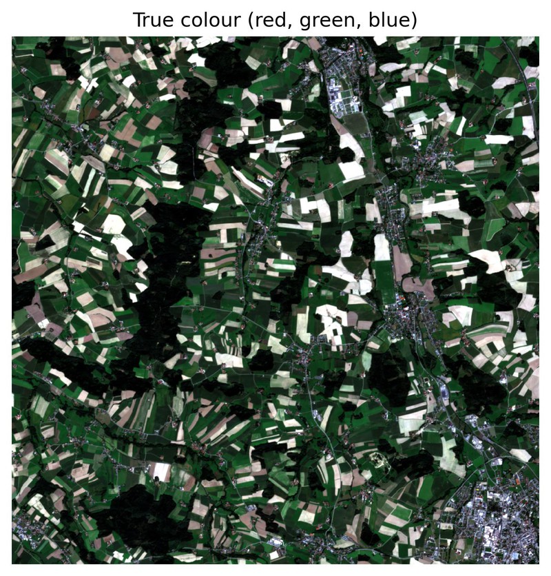
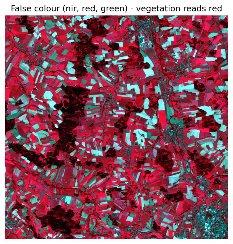
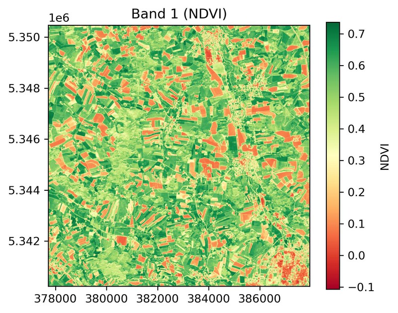
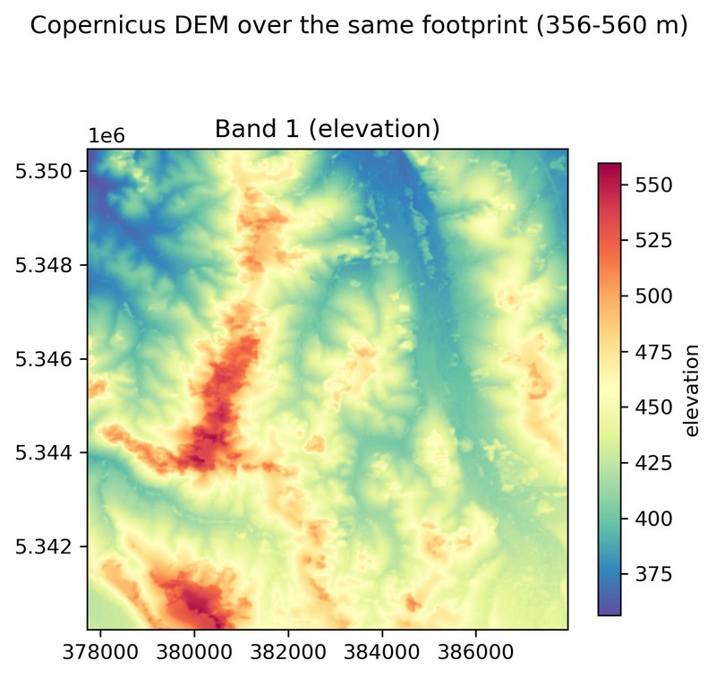
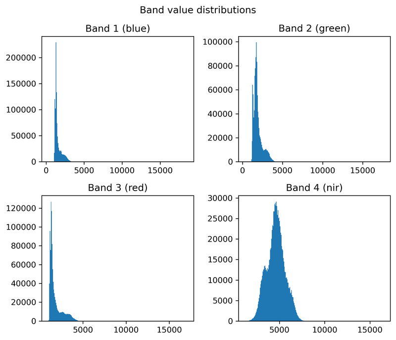
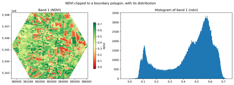
Every image below is straight out of an Easy-EO plotting call on the sample
dataset, with the library's own defaults - no touch-ups. Regenerate them all
with python scripts/build_gallery.py.
 |
 |
scene.plot_composite(["red", "green", "blue"]) |
scene.plot_composite(["nir", "red", "green"]) |
 |
 |
scene.ndvi(red="red", nir="nir", name="NDVI").plot_raster(cmap="RdYlGn") |
dem.plot_raster(cmap="Spectral_r") - the same call on a DEM |
 |
 |
scene.plot_histogram() - every band at once |
clipped.plot_raster_with_histogram(cmap="RdYlGn") |
Bands are addressed by name throughout ("red", "nir") because the sample
carries band descriptions; a 1-based index works anywhere a name does.
Supported Backends
| Backend | Description |
|---|---|
| NumPy | Fast, in-memory arrays without I/O |
| Rasterio | Full geospatial support (CRS, transform, resampling) |
Documentation
📚 Full documentation is available at:
Project Status
🚧 Active development The API is stabilizing but may change before v1.0.
Contributing
Contributions are welcome!
- Bug reports
- Feature requests
- Documentation improvements
Please open an issue or pull request on GitHub.
License
MIT License © 2025 Thomas Burns Botchwey
1 maintainer

Download files
Download the file for your platform. If you're not sure which to choose, learn more about installing packages.
Source Distribution
Built Distribution
Filter files by name, interpreter, ABI, and platform.
If you're not sure about the file name format, learn more about wheel file names.
Copy a direct link to the current filters
File details
Details for the file easy_eo-0.3.1.tar.gz.
File metadata
- Download URL: easy_eo-0.3.1.tar.gz
- Upload date:
- Size: 84.7 kB
- Tags: Source
- Uploaded using Trusted Publishing? Yes
- Uploaded via:
twine/7.0.0 CPython/3.13.14
File hashes
| Algorithm | Hash digest | |
|---|---|---|
| SHA256 |
0ba5254ba9cef1f504ddec284091a7c0f94b176667cb506d4d2b6286306bde36
|
|
| MD5 |
0e705824510f012bd9d910cfd592ea5a
|
|
| BLAKE2b-256 |
18b6c804754d056f249ca88eb70c5d5c125615fb7c87e5ef82be14d891764f03
|
Provenance
The following attestation bundles were made for easy_eo-0.3.1.tar.gz:
Publisher:
release.yml on Tommy-Burns/easy-eo
-
Statement:
-
Statement type:
https://in-toto.io/Statement/v1 -
Predicate type:
https://docs.pypi.org/attestations/publish/v1 -
Subject name:
easy_eo-0.3.1.tar.gz -
Subject digest:
0ba5254ba9cef1f504ddec284091a7c0f94b176667cb506d4d2b6286306bde36 - Sigstore transparency entry: 2489751479
- Sigstore integration time:
-
Permalink:
Tommy-Burns/easy-eo@7cf9dbb6159f6935a3bfad894a494c9dafe2875d -
Branch / Tag:
refs/tags/v0.3.1 - Owner: https://github.com/Tommy-Burns
-
Access:
public
-
Token Issuer:
https://token.actions.githubusercontent.com -
Runner Environment:
github-hosted -
Publication workflow:
release.yml@7cf9dbb6159f6935a3bfad894a494c9dafe2875d -
Trigger Event:
push
-
Statement type:
File details
Details for the file easy_eo-0.3.1-py3-none-any.whl.
File metadata
- Download URL: easy_eo-0.3.1-py3-none-any.whl
- Upload date:
- Size: 100.3 kB
- Tags: Python 3
- Uploaded using Trusted Publishing? Yes
- Uploaded via:
twine/7.0.0 CPython/3.13.14
File hashes
| Algorithm | Hash digest | |
|---|---|---|
| SHA256 |
fa010a86449d09ebb4e928a120b250ceef88ded1d93807c1151cd2c9cc05b427
|
|
| MD5 |
12d27fa9dc25606db2cc71577dff5e75
|
|
| BLAKE2b-256 |
9067b7f494299aa68b73b9c371d89d8945524d2656d9ac5a2d62e13ee1087888
|
Provenance
The following attestation bundles were made for easy_eo-0.3.1-py3-none-any.whl:
Publisher:
release.yml on Tommy-Burns/easy-eo
-
Statement:
-
Statement type:
https://in-toto.io/Statement/v1 -
Predicate type:
https://docs.pypi.org/attestations/publish/v1 -
Subject name:
easy_eo-0.3.1-py3-none-any.whl -
Subject digest:
fa010a86449d09ebb4e928a120b250ceef88ded1d93807c1151cd2c9cc05b427 - Sigstore transparency entry: 2489751503
- Sigstore integration time:
-
Permalink:
Tommy-Burns/easy-eo@7cf9dbb6159f6935a3bfad894a494c9dafe2875d -
Branch / Tag:
refs/tags/v0.3.1 - Owner: https://github.com/Tommy-Burns
-
Access:
public
-
Token Issuer:
https://token.actions.githubusercontent.com -
Runner Environment:
github-hosted -
Publication workflow:
release.yml@7cf9dbb6159f6935a3bfad894a494c9dafe2875d -
Trigger Event:
push
-
Statement type:














