
EasyPred: track your predictions with ease






What is it?
EasyPred is a Python package to easily store, analyse, assess and compare predictions from Machine Learning and Data Mining models.
The package allows to create different types of model-agnostic prediction objects simply by passing real and fitted data. These objects have properties and methods that return various accuracy and error metrics, together with relevant plots.
Why EasyPred can be useful:
- All-in-one bundle: having data and accuracy metrics in a single object means less stuff you need to keep an eye on
- Minimize code redundancy: pass the data once and get all the information and metrics you want
- Easy and flexible comparison: create the predictions first and then decide what to compare. Changed your mind? The object is there, simply access another method
Quick Start
Installation
You can install EasyPred via pip
pip install easypred
Alternatively, you can install EasyPred by cloning the project to your local directory
git clone https://github.com/FilippoPisello/EasyPred
And then run setup.py
python setup.py install
Usage
At the moment, three types of predictions are implemented:
- Prediction: any prediction
- BinaryPrediction: fitted and real data attain only two values
- NumericPrediction: fitted and real data are numeric
Then there is the case when observations are matched to a probability rather than to an outcome:
- BinaryScore: prediction output that returns probability scores
Prediction
Consider the example of a generic prediction over text categories:
>>> real_data = ["Foo", "Foo", "Bar", "Bar", "Baz"]
>>> fitted_data = ["Baz", "Bar", "Foo", "Bar", "Bar"]

>>> from easypred import Prediction
>>> pred = Prediction(real_data, fitted_data)
Let's check the rate of correctly classified observations:
>>> pred.accuracy_score
0.2
More detail is needed, let's investigate where predictions and real match:
>>> pred.matches()
array([False, False, False,  True, False])
Still not clear enough, display everything in a data frame:
>>> pred.as_dataframe()
  Real Values Fitted Values  Prediction Matches
0         Foo           Baz               False
1         Foo           Bar               False
2         Bar           Foo               False
3         Bar           Bar                True
4         Baz           Bar               False
BinaryPrediction
Consider the case of a classic binary context (note: the two values can be any value, no need to be 0 and 1):
>>> real_data = [1, 1, 0, 0]
>>> fitted_data = [0, 1, 0, 0]
>>> from easypred import BinaryPrediction
>>> bin_pred = BinaryPrediction(real_data, fitted_data, value_positive=1)
What are the false positive and false negative rates? What about sensitivity and specificity?
>>> bin_pred.false_positive_rate
0.0
>>> bin_pred.false_negative_rate
0.5
>>> bin_pred.recall_score
0.5
>>> bin_pred.specificity_score
1.0
Let's look now at the confusion matrix as a pandas data frame:
>>> bin_pred.confusion_matrix(as_dataframe=True)
        Pred 0  Pred 1
Real 0       2       0
Real 1       1       1
NumericPrediction
Let's look at the numeric use case:
>>> real_data = [1, 2, 3, 4, 5, 6, 7]
>>> fitted_data = [1, 2, 4, 3, 7, 2, 5]
>>> from easypred import NumericPrediction
>>> num_pred = NumericPrediction(real_data, fitted_data)
We can access the residuals with various flavours, let's go for the basic values:
>>> num_pred.residuals(squared=False, absolute=False, relative=False)
array([ 0,  0, -1,  1, -2,  4,  2])
The data frame representation has now more information:
>>> num_pred.as_dataframe()
   Fitted Values  Real Values  Prediction Matches  Absolute Difference  Relative Difference
0              1            1                True                    0             0.000000
1              2            2                True                    0             0.000000
2              4            3               False                   -1            -0.333333
3              3            4               False                    1             0.250000
4              7            5               False                   -2            -0.400000
5              2            6               False                    4             0.666667
6              5            7               False                    2             0.285714
There are then a number of dedicated error and accuracy metrics:
>>> num_pred.mae
1.4285714285714286
>>> num_pred.mse
3.7142857142857144
>>> num_pred.rmse
1.927248223318863
>>> num_pred.mape
0.27653061224489794
>>> num_pred.r_squared
0.31250000000000017
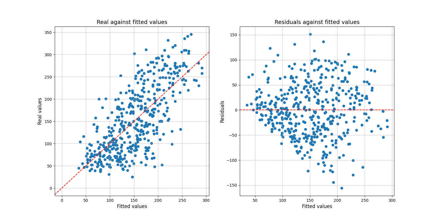
For a more complex scenario one may be interested into visualizing the residuals and prediction fit:
# Setting up the example, creating the prediction
>>> from sklearn import datasets, linear_model
>>> diabetes_X, diabetes_y = datasets.load_diabetes(return_X_y=True)
>>> regr = linear_model.LinearRegression()
>>> regr.fit(diabetes_X, diabetes_y)
LinearRegression()
>>> diabetes_y_pred = regr.predict(diabetes_X)
# Loading the prediction into easypred
>>> from easypred import NumericPrediction
>>> pred = NumericPrediction(diabetes_y, diabetes_y_pred)
>>> pred.plot_fit_residuals()
array([<AxesSubplot:title={'center':'Real against fitted values'},
       xlabel='Fitted values', ylabel='Real values'>,
       <AxesSubplot:title={'center':'Residuals against fitted values'},
       xlabel='Fitted values', ylabel='Residuals'>],
      dtype=object)
>>> from matplotlib import pyplot as plt
>>> plt.show()
BinaryScore
BinaryScore is to be used when working with probability scores, generally assigned in a 0-1 interval displaying the likelihood of an observation "of being 1".
Here using one of Sklearn's datasets:
>>> from sklearn.datasets import load_breast_cancer
>>> from sklearn.linear_model import LogisticRegression
>>> X, y = load_breast_cancer(return_X_y=True)
>>> clf = LogisticRegression(solver="liblinear", random_state=0).fit(X, y)
>>> probs = clf.predict_proba(X)[:, 1]
>>> from easypred import BinaryScore
>>> score = BinaryScore(y, probs, value_positive=1)
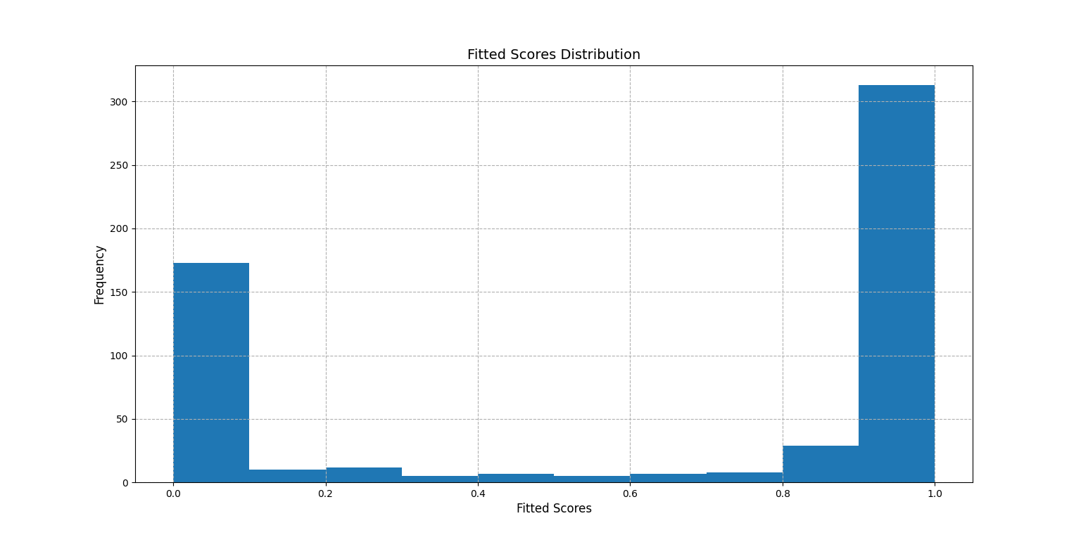
First we visualize the distribution of the fitted scores:
>>> score.plot_score_histogram()
<AxesSubplot:title={'center':'Fitted Scores Distribution'}, xlabel='Fitted Scores', ylabel='Frequency'>
>>> from matplotlib import pyplot as plt
>>> plt.show()
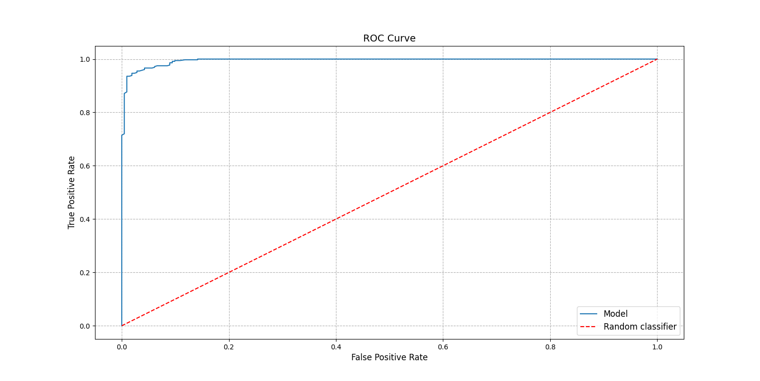
A key metric in this case is the AUC score:
>>> score.auc_score
0.9947611119919667
To better understand the number the ROC curve can be plotted:
>>> score.plot_roc_curve()
<AxesSubplot:title={'center':'ROC Curve'}, xlabel='False Positive Rate', ylabel='True Positive Rate'>
>>> plt.show()
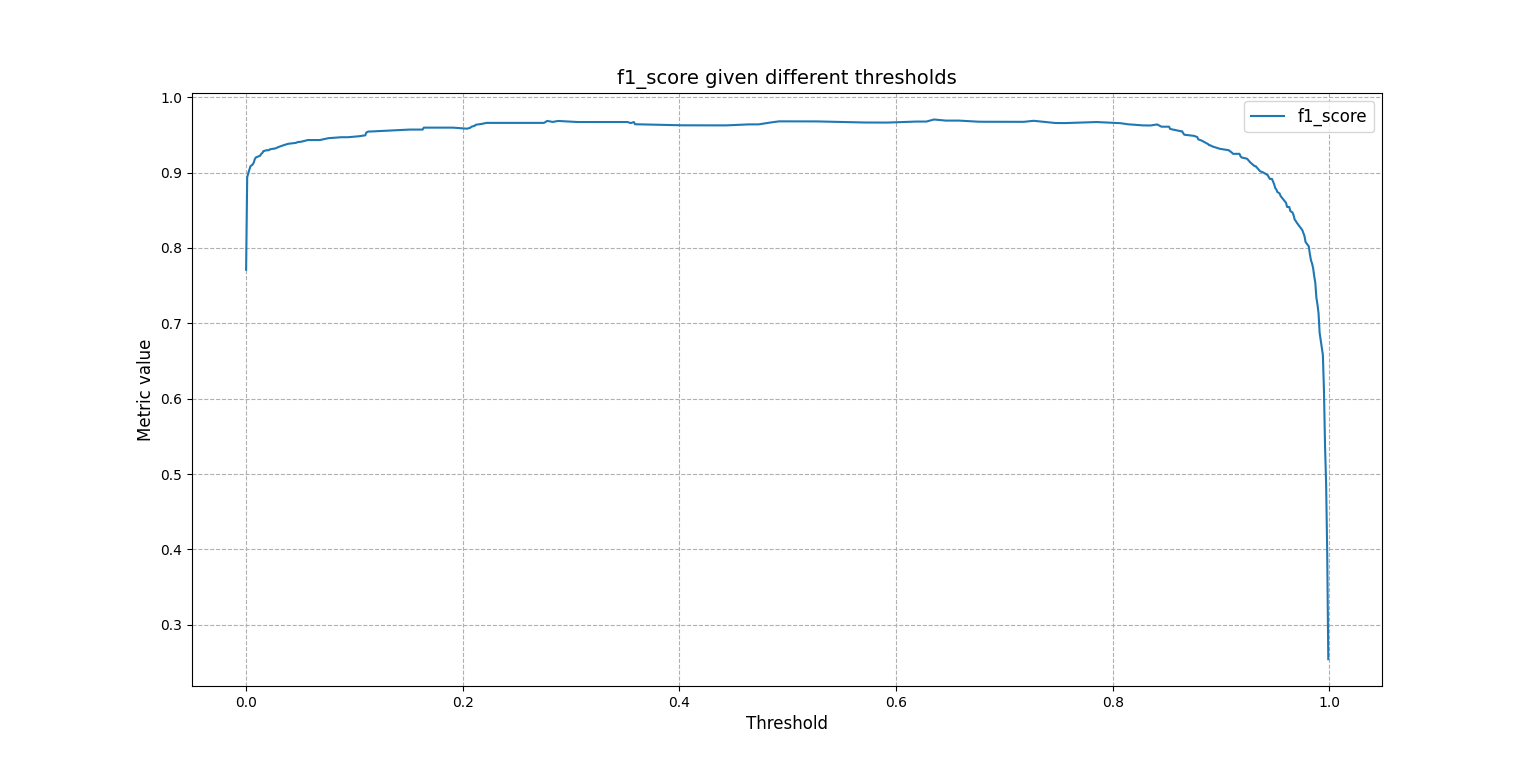
Or one may want to know how the F1 score changes as the threshold to tell 1s from 0s takes different values:
>>> score.f1_scores
array([0.77105832, 0.89361702, 0.89924433, 0.90379747, ...])
The same array can be plotted for a visual understanding:
>>> from easypred.metrics import f1_score
>>> score.plot_metric(f1_score)
<AxesSubplot:title={'center':'f1_score given different thresholds'}, xlabel='Threshold', ylabel='Metric value'>
>>> plt.show()
To get a summary:
>>> score.describe()
                          Value
N                    569.000000
Max fitted score       0.999996
AUC score              0.994761
Max accuracy           0.963093
Thresh max accuracy    0.635000
Max F1 score           0.970464
Thresh max F1 score    0.635000
Dependencies
EasyPred depends on the following libraries:
- NumPy
- pandas
- matplotlib
Documentation
Find the complete documentation on read the docs.
License
1 maintainer

Metadata
1 maintainer
Release files for easypred 0.1.4
For a detailed explanation of source distributions (sdists) and built distributions (wheels), please see the package formats documentation.
Source distribution (sdist)
| File | Size | Uploaded | |
|---|---|---|---|
| easypred-0.1.4.tar.gz | 54.5 kB | Details |
Built distribution (wheel)
| File | Interpreter | ABI | Platform | Reset |
|---|---|---|---|---|
| easypred-0.1.4-py3-none-any.whl | Python 3 | none | any | Details |
Total release size: 110.9 kB
Release files / easypred-0.1.4.tar.gz
| Download URL | easypred-0.1.4.tar.gz |
|---|---|
| Size | 54.5 kB |
| Tags | Source |
|
SHA-256 checksum How to use checksums |
1287514004926afd670804a74b8f7c48c9d251f3c4f197143c298dcb90d724bd
|
|
BLAKE2b-256 checksum How to use checksums |
bb3a250dd3826f97f36f24f2018ecb4252d8c269d5b3833ae809ced42090598e
|
| Upload date | |
|
Uploaded using Trusted Publishing? What is trusted publishing? |
No |
| Uploaded via |
twine/3.7.1 importlib_metadata/4.10.0 pkginfo/1.8.2 requests/2.26.0 requests-toolbelt/0.9.1 tqdm/4.62.3 CPython/3.9.9
|
Release files / easypred-0.1.4-py3-none-any.whl
| Download URL | easypred-0.1.4-py3-none-any.whl |
|---|---|
| Size | 56.5 kB |
| Tags | Python 3 |
|
SHA-256 checksum How to use checksums |
5452ba80b6e2e30b5af0c313d172cbbf18db1304ad6116e8c70eb2700df2030a
|
|
BLAKE2b-256 checksum How to use checksums |
d1b66f2aec2e9956ae0b1956f057b73138d34fefa284005daf0572701fe98915
|
| Upload date | |
|
Uploaded using Trusted Publishing? What is trusted publishing? |
No |
| Uploaded via |
twine/3.7.1 importlib_metadata/4.10.0 pkginfo/1.8.2 requests/2.26.0 requests-toolbelt/0.9.1 tqdm/4.62.3 CPython/3.9.9
|














