
EBF — Elliptical Basis Function Interpolation
Extract smooth functional relationships from scattered, arbitrarily-dimensioned engineering data. EBF generalizes Radial Basis Function (RBF) interpolation by giving every node its own learnable ellipsoid instead of a single shared spherical radius — so instead of assuming what "distance" means between your variables, the model learns it.
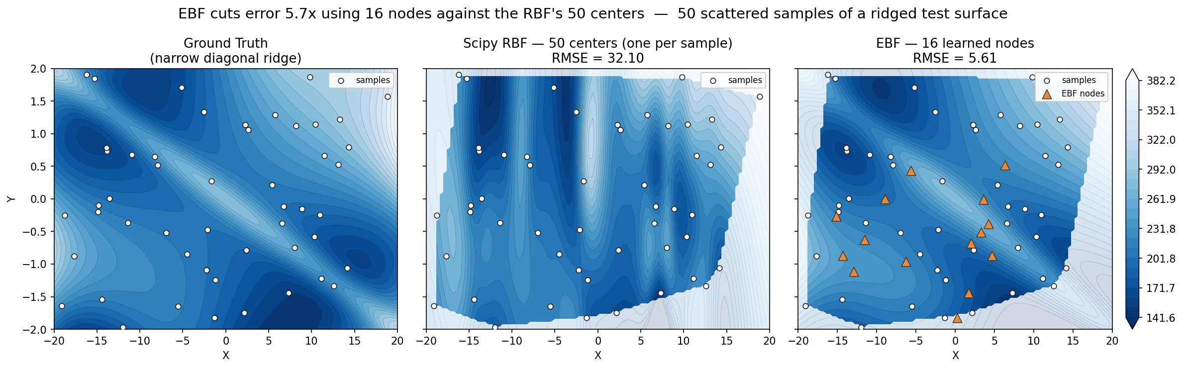
50 scattered samples of a surface with a narrow diagonal ridge. Scipy's RBF places a center
at every sample (50 of them) and still rings around the ridge — RMSE 32.10. EBF uses 16
learned nodes and follows it — RMSE 5.61. Both are scored against ground truth inside the
convex hull of the samples; the faint regions outside it are extrapolation, shown for
context. Reproduce with examples/RBF_vs_EBF.py.
What Makes It Different
A conventional RBF measures distance from every center with one shared, circular metric, so
a center can only ever cover a round patch. An EBF node carries its own positive-definite
matrix Aᵢ, and the optimizer is free to stretch and rotate it during training.
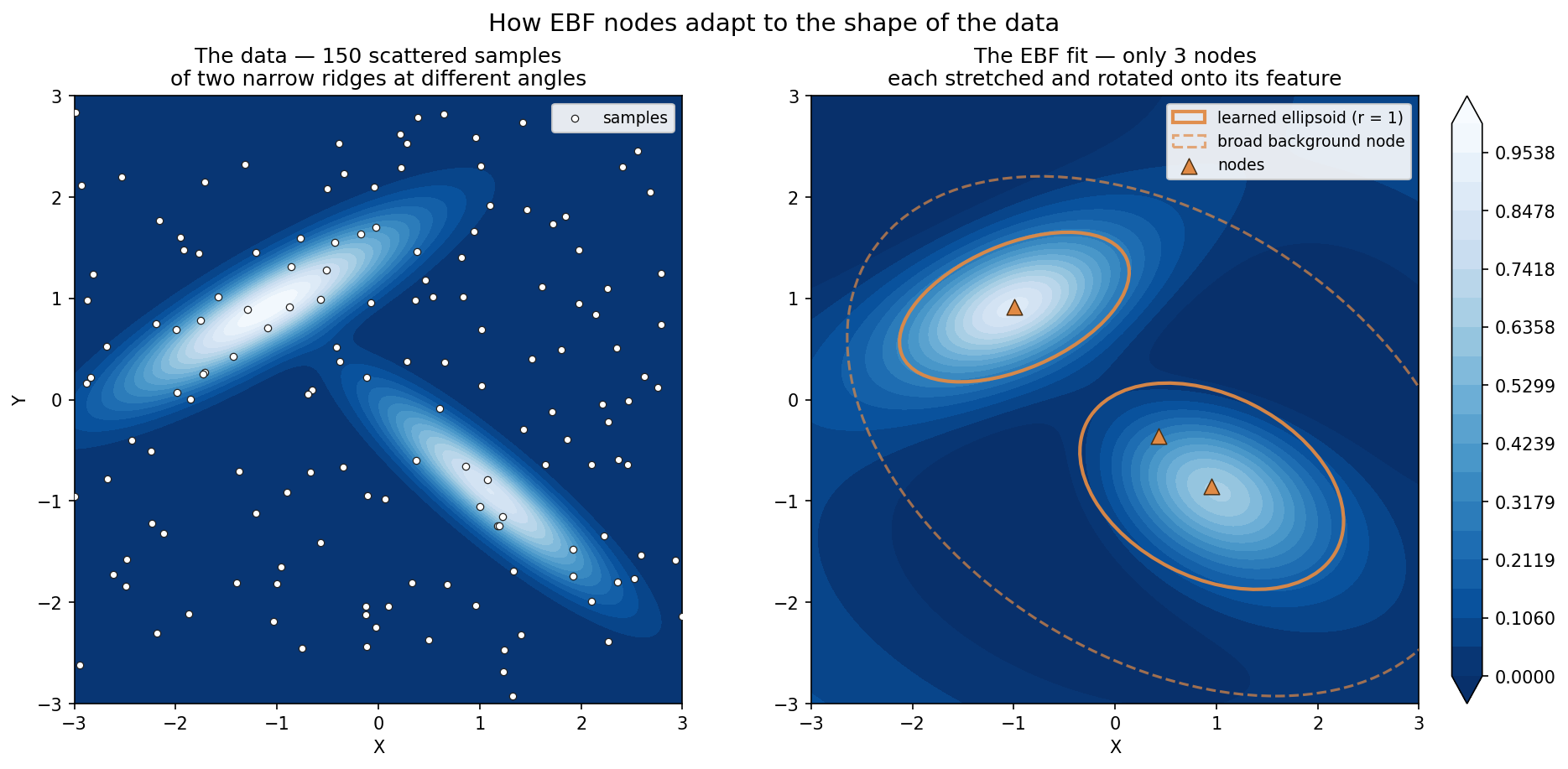
Three nodes fit to two narrow ridges at +30° and −40°. Two nodes elongate and turn onto a
ridge each; the third stays broad and carries the background. Nothing instructs the model to
do this — it falls out of minimizing fit error. Reproduce with
examples/node_ellipsoids.py.
The model equation:
ŷ = Σᵢ aᵢ · φ(rᵢ²) + b₁·x + b₂
where rᵢ² = (x − vᵢ)ᵀ Aᵢ (x − vᵢ) and each Aᵢ = LᵢLᵢᵀ + εI is guaranteed positive-definite
via Cholesky factorization. A global linear trend term captures broad gradients, while the
basis function sum captures nonlinear detail.
See ALGORITHM.md for the full derivation.
Why This Matters More As Dimensions Grow
RBF interpolation carries an assumption inherited from the spatial problems it was invented for: that the input space is Euclidean, so distance means something. For latitude and longitude that holds — two points a kilometre apart are physically related, and a circular kernel encodes that correctly.
Engineering data rarely works this way. When your axes are speed, power, temperature, pressure, mass, and price, there is no common unit and therefore no natural notion of distance. How far is 10 kPa from 3 °C? Standardizing each axis to unit variance — which EBF does automatically — supplies a default answer, but that is a guess, not a physical fact.
The per-node ellipsoid is that guess made learnable. Rather than assuming a metric, the
optimizer infers one from the data. And because each Aᵢ is a full symmetric matrix rather
than a per-axis scaling, it can rotate as well as stretch — so the model can capture that two
variables act together, not just that one matters more than another. Each node carries its
own, so the inferred relationship is free to differ across the space: the metric that fits
one operating region need not be the metric that fits another.
This is why the advantage tends to widen with dimensionality. In 2-D you can often eyeball a sensible scaling; in 6-D, with mixed units and interactions, you generally cannot.
Features
- Per-node learnable ellipsoids — each node adapts its own anisotropic distance metric
- Any number of inputs — 1-D, 2-D, or 20-D; the fit, export, and diagnostics don't care
- 12 basis functions — multiquadric (default), Gaussian, Matern, thin plate, cubic, and more
- Robust losses — Huber downweights outliers, Tukey rejects them outright; both self-calibrate to the residual noise floor
- Automatic data standardization — inputs and outputs are scaled internally; predictions come back in original units
- Early stopping — optional validation split with best-weight restore
- Visualization and export — diagnostic plots, contour maps, and CSV/NPZ lookup tables
- Save/load — TensorFlow checkpoints with a JSON sidecar for full reproducibility
Installation
pip install ebf
or with poetry:
poetry add ebf
Requires Python >= 3.11. TensorFlow, numpy, scipy, matplotlib and cmasher install automatically. The example scripts additionally need pandas and openpyxl:
pip install "ebf[examples]"
For a development install, see Contributing.
Quick Start
Akima's benchmark dataset — a long flat run followed by a steep rise, where splines tend to overshoot:
import numpy as np
import ebf

x = np.array([0, 2, 3, 5, 6, 8, 9, 11, 12, 14, 15], dtype=float)
y = np.array([10, 10, 10, 10, 10, 10, 10.5, 15, 50, 60, 85])
X = x.reshape(-1, 1)                 # inputs are always 2-D: (n_points, n_dims)

model = ebf.EBF(n_nodes=11)
model.fit(X, y, steps=20000, var_weight=0.5, seed=42)

# Predict anywhere — not just at the training points
query = np.linspace(x.min(), x.max(), 200).reshape(-1, 1)
y_fit = model.predict(query)
Full script: examples/1d_fit.py.
Data contract: inputs are (n_points, n_dims) and outputs (n_points,). You can also
pass a single combined (n_points, n_dims+1) array, in which case the last column is
always the output:
data = np.column_stack([x1, x2, y])
model.fit(data)                      # last column treated as the output
Typical Workflow
Fit, check the fit, look at the surface, export it. Every plotting helper accepts an ax=
argument so you can compose figures, and returns (fig, ax).
import ebf

# 1. Fit
model = ebf.EBF(n_nodes=16, basis='multiquadric')
model.fit(X, y, steps=60000, var_weight=0.1, seed=42)

# 2. Diagnose — did it converge, and is the fit any good?
ebf.convergence_plot(model)          # loss curve from model.history_
ebf.correlation_plot(y, model.predict(X))   # data vs prediction, with R²
ebf.residual_plot(y, model.predict(X))      # bias trends and outliers

# 3. Inspect the surface (2-D inputs)
ebf.contour_plot_2d(model, X, y, show_nodes=True,
                    xlabel='X1', ylabel='X2', zlabel='Y')

# 4. Or get all four diagnostics in one figure
ebf.summary_plot_3d(model, X, y, xlabel='X1', ylabel='X2', zlabel='Y')

# 5. Export a lookup table for use elsewhere
bounds = list(zip(X.min(axis=0), X.max(axis=0)))
grid = ebf.eval_grid(model, bounds, n_points=100)
ebf.export_grid("lookup.csv", grid, dim_names=['X1', 'X2'])
eval_grid() works in any number of dimensions; export_grid() writes .csv (portable) or
.npz (compact, full precision). Contour plots mask everything outside the convex hull of
your training data by default, so you don't mistake extrapolation for a fit.
Full details in docs/visualization.md.
One figure, whole fit
summary_plot_3d() is step 4 above — it composes the surface and all three diagnostics into
a single figure. This is a compressor efficiency map: 56 operating points, 9 nodes.
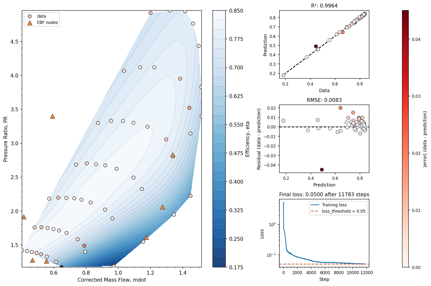
Left: the fitted efficiency surface, with training data and the learned node positions
(orange triangles). Right, top to bottom: prediction vs data with R² = 0.9964; residuals
vs prediction, RMSE 0.0083 — about 1.3% of the 0.184–0.843 efficiency range, with one point
standing clearly apart; and the training loss, which hit its loss_threshold after 11,783 of
the 80,000 requested steps. Every data point is shaded by its absolute error on one shared
red scale (colorbar, far right), so the same shade means the same error on all three panels.
Reproduce with examples/comp_map_ebf.py.
Read together these answer the three questions worth asking of any fit: is it accurate (correlation), is it wrong anywhere in particular (residuals), and did it actually converge (loss curve). The residual panel is the one that earns its keep — that single outlier near prediction 0.5 is invisible on the correlation plot, which compresses it against the 1:1 line. The shared error shading then places it: it is the darkest point on the map, in the low-flow, low-pressure-ratio corner where the data thins out.
Inspecting what was learned
nodes = model.get_nodes()            # (n_nodes, n_dims) centers, original units
A     = model.get_ellipsoids()       # (n_nodes, n_dims, n_dims) ellipsoid matrices
imp   = model.get_node_importance(X_holdout, y_holdout)   # (n_nodes,) RMSE cost of dropping each
get_ellipsoids() returns the Aᵢ in the same units as get_nodes(), so the two compose
directly — eigen-decompose A to recover each node's axis lengths and orientation.
get_node_importance() drops each node in turn and re-solves the remaining amplitudes in
closed form, reporting how much RMSE degrades in original output units. The refit is the
whole point: with a growing basis, nodes represent features by cancelling against each
other, so simply zeroing one vastly overstates its importance. Near-zero entries mark nodes
whose job the others can absorb. Pass held-out data — importance measured on unseen points
is the more honest signal.
Working in Any Number of Dimensions
The examples in this repository are almost all 2-D because two inputs and one output are
what a contour plot can show — not because the method is limited to them. Fitting is
dimension-agnostic: n_dims is inferred from your data, and nothing in the model, the
training loop, or the export path assumes a particular count.
# 5 inputs -> 1 output, no different from the 2-D case
X = measurements[:, :5]        # speed, power, temperature, pressure, mass
y = measurements[:, 5]         # the quantity you care about

model = ebf.EBF(n_nodes=24)
model.fit(X, y, steps=60000, seed=42)

y_hat = model.predict(X_new)   # (n_points, 5) in, (n_points,) out
A     = model.get_ellipsoids() # (24, 5, 5) — the learned metric per node
What changes with dimensionality is only what you can draw:
| Capability | Dimensions |
|---|---|
fit, predict, get_nodes, get_ellipsoids, save/load |
any |
convergence_plot, correlation_plot, residual_plot |
any |
eval_grid, export_grid |
any |
contour_plot_2d |
2 inputs only |
summary_plot_3d |
2 inputs + 1 output only |
Above two inputs, lean on correlation_plot and residual_plot — they judge fit quality
from paired arrays and never need to see the input space. To look at a high-dimensional
surface, hold the other inputs fixed and sweep two of them with eval_grid, which produces
a 2-D slice you can contour.
Grid size grows exponentially.
eval_gridevaluatesn_points ** n_dimslocations. The 100×100 grid that is routine in 2-D becomes 10¹⁰ points in 5-D. Use a coarsen_points, or pass a list to set the resolution per dimension and spend it only where the response actually varies.
The low end
1-D works too, and examples/1d_fit.py demonstrates it — though it is
admittedly overkill. With a single input there is no cross-dimensional relationship left to
learn, so each ellipsoid collapses to a scalar width and EBF reduces to something close to a
conventional RBF. The one thing you still gain is that node locations are trainable, so
centers migrate toward the regions that need them rather than sitting where you put them.
The interesting case is the other direction.
Choosing Parameters
Constructor (ebf.EBF(...)):
| Parameter | Default | Description |
|---|---|---|
n_nodes |
— | Number of EBF nodes (more nodes = more detail) |
basis |
'multiquadric' |
Basis function name — see Basis Functions |
eps |
1e-8 | Numerical stability offset (only cosh / inv_cosh use it) |
Training (model.fit(...)):
| Parameter | Default | Description |
|---|---|---|
steps |
60000 | Training iterations |
lr |
0.01 | Initial Adam learning rate (decays exponentially) |
var_weight |
0.2 | Node spread regularization — higher values produce smoother fits |
ellipsoid_weight |
0.0 | Ellipsoid shape penalty — the explicit smoothness knob; 0 disables it |
loss_type |
'rmse' |
'rmse', 'huber' (downweights outliers), or 'tukey' (rejects outliers) |
huber_delta |
'auto' |
Huber threshold — 'auto' (1.345σ) tracks the residual noise floor; '<k>sigma' sets K yourself; a float fixes it |
tukey_c |
'auto' |
Tukey rejection point — residuals beyond it exert zero pull; 'auto' (4.685σ) or e.g. '3sigma' to reject harder |
val_fraction |
0.0 | Held-out fraction for early stopping; 0 disables. Needs ~50+ points |
patience |
10 | Validation evaluations (1 per 100 steps) without improvement before stopping |
loss_threshold |
None | Stop early once the training loss reaches this value; None disables |
verbose |
True | Print training progress every 100 steps |
seed |
None | Set for reproducible results |
Start here: n_nodes at roughly 1/3 to 1/2 your point count, everything else default.
This holds for the default multiquadric and other growing bases; if you switch to a
decaying basis, start lower — see How many nodes?.
Then:
| Symptom | Try |
|---|---|
| Surface is too wiggly / chases noise | Raise ellipsoid_weight (start at 0.001), then var_weight; with a decaying basis, cut n_nodes first |
| Surface is too flat, misses real features | Lower var_weight, add nodes |
| Nodes visibly cluster on top of each other | Raise var_weight |
| A few bad measurements drag the surface | loss_type='huber' |
| Some points are outright wrong | loss_type='tukey' |
| Loss still falling at the last step | Raise steps |
| Noisy data, unsure when to stop | val_fraction=0.15 (needs ~50+ points) |
var_weight and ellipsoid_weight are the two smoothing knobs. var_weight pushes nodes
apart, which broadens their influence zones indirectly; ellipsoid_weight penalizes sharp
ellipsoids directly, so reach for it first when a fit is too wiggly.
How many nodes? It depends on the basis
Over-specifying n_nodes is not equally dangerous for every basis, because the two basis
families fail differently when given surplus capacity:
- Growing bases (
multiquadric,cubic,thin_plate,linear,quadratic,cosh) increase with distance, so every node influences every point. Local features are built by cancellation between nodes, and there is no way to raise a private spike over a single data point. Surplus nodes go into near-collinear directions that leave the surface smooth. - Decaying bases (
gaussian,matern32,matern52,inv_quadratic,inv_multiquadric,inv_cosh) fall to zero with distance, so each node owns a neighborhood and is a local feature in its own right. With one node per sample, every point can get its own bump — and the model can interpolate the noise exactly.
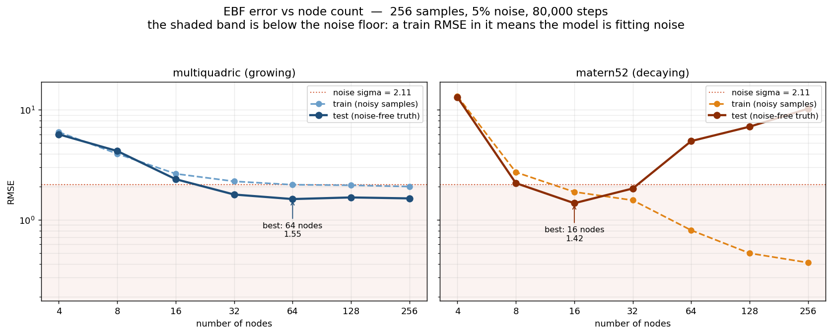
examples/node_count_gallery.py sweeps both from 4 nodes
to one node per sample — 256 samples of a ridged surface with 5% noise (σ = 2.11), trained
to convergence at 80,000 steps. The rightmost column is 1539 parameters against 256
observations.
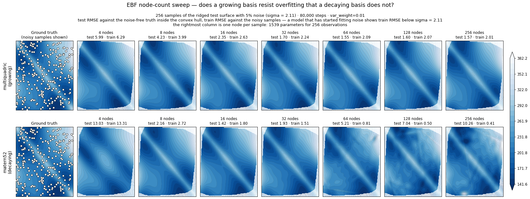
The top row barely changes past 32 nodes. The bottom row visibly breaks up from 64 nodes onward — those blotches are nodes sitting on individual samples and chasing their noise.
| basis | family | best test RMSE | at 256 nodes | penalty | train RMSE at 256 |
|---|---|---|---|---|---|
multiquadric |
growing | 1.55 (64 nodes) | 1.57 | 1.01× | 2.01 — at the noise floor |
matern52 |
decaying | 1.42 (16 nodes) | 10.26 | 7.2× | 0.41 — a fifth of σ |
The growing basis is essentially flat once it has enough nodes: 64 or 256 makes no difference worth the compute. The decaying basis has a sharp optimum and degrades hard past it, and its training error keeps falling below the noise floor the whole way — the signature of a model fitting noise rather than signal.
Two things this depends on, both easy to miss:
- A decaying basis turns early — well before one node per sample.
matern52is already past its optimum at 32 nodes (ratio 0.125) and 3.4× worse by 64. The blowup at the far end is the dramatic version, but the damage starts much sooner than "extreme" would suggest. - The model has to actually reach capacity. Gradient descent from a small initialization over a finite step budget is itself a regularizer, and a model that stopped before fitting the signal cannot demonstrate anything about overfitting — at a short step budget both families look equally well behaved. Read training RMSE against the noise floor: a model chasing noise sits below σ. If it sits above, you are measuring how far Adam got, not what the node count does.
What to do with this:
- With the default
multiquadric— or any growing basis — the 1/3 to 1/2 rule above holds, and erring high is cheap. This is the main reason it is the default. - With a decaying basis, the rule does not hold: at 1/3 of 256 points
matern52is already ~5× worse than its best. Start lower, around 1/10 of your point count, and tune upward while watching held-out error rather than training error. - Either way, compare training RMSE against your expected noise level. If it has dropped
well below, the surface is fitting measurement noise no matter how good the training number
looks.
val_fraction=0.15catches this automatically.
Measured on one synthetic 2-D surface, one noise level and two of the twelve basis functions — chosen as clear representatives of each family. Each node costs
1 + n_dims + n_dims(n_dims+1)/2parameters, so how fast you reach the over-parameterized regime is dimension-dependent, and the node counts above will not transfer directly to your data. Treat the direction as the finding, and the specific crossover point as something to check on your own held-out set. Reproduce or extend withpython examples/node_count_gallery.py --save-only.
Robust Fitting
Real measurements contain noise and the occasional bad point. loss_type controls how hard
a residual pulls on the surface.
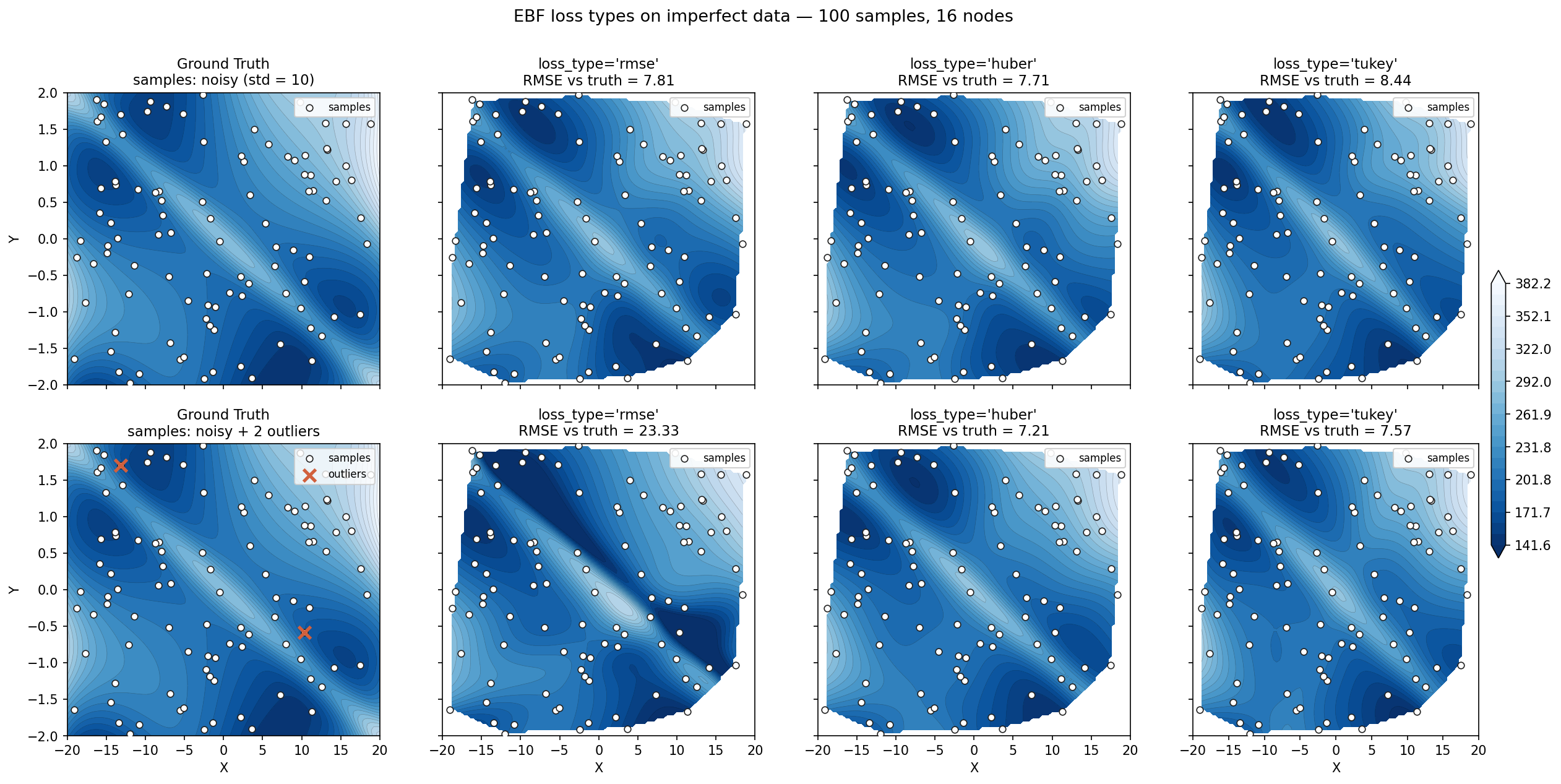
Same surface, fit three ways under two corruption scenarios, each scored against clean
ground truth. With noise alone all three land within ~10% of each other (rmse 7.81, huber
7.71, tukey 8.44). Add just two gross outliers and squared error collapses — RMSE 23.33,
with a visible gash torn across the surface — while both robust losses hold near 7.2 (huber
7.21, tukey 7.57). Reproduce with examples/loss_comparison.py.
Huber is the sensible default. It was at least as good as Tukey in both scenarios above
and degrades gracefully. Tukey earns its keep when outliers are numerous or extreme enough
that even Huber's bounded pull still drags the surface. Both thresholds self-calibrate from
the residual spread when left at 'auto'.
Basis Functions
Select a basis function by name when creating the model:
model = ebf.EBF(n_nodes=16, basis='gaussian')
| Name | Expression |
|---|---|
multiquadric (default) |
a₁ · (√(r²+1) − 1) |
gaussian |
a₁ · exp(−r²) |
linear |
a₁ · r |
quadratic |
a₁ · r² |
cubic |
a₁ · r³ |
thin_plate |
a₁ · r² ln(r²) |
inv_multiquadric |
a₁ / √(r²+1) |
inv_quadratic |
a₁ / (1+r²) |
matern32 |
a₁ · (1+√3·r) · exp(−√3·r) |
matern52 |
a₁ · (1+√5·r+⅗r²) · exp(−√5·r) |
cosh |
a₁ · cosh(√(r²+ε)) |
inv_cosh |
a₁ / cosh(√(r²+ε)) |
Growing functions (multiquadric, linear, quadratic, cubic, thin_plate, cosh)
give every node global reach. Decaying functions (gaussian, inv_*, matern*) keep
node influence local, which limits wild extrapolation outside the data hull.
That locality cuts both ways: it is what tames extrapolation, and also what lets surplus nodes chase noise inside the hull. A decaying basis needs its node count chosen with more care and is far less forgiving of guessing high — see How many nodes?.
See docs/basis_functions.md for the visual gallery and guidance.
Saving and Loading
ckpt = model.save("checkpoints/", filename="my-model")

model = ebf.EBF.load(ckpt)           # returns a fitted EBF instance
y_pred = model.predict(X_new)
The checkpoint stores the weights, the basis configuration, and the Scale/Offset values needed to move between scaled and original units.
Functional API
A lower-level interface is also available for callers that prefer to manage state themselves:
Scale, Offset, file = ebf.run(data, n_nodes=32, train_steps=20000)
predictions, nodes = ebf.run_points(data[:, :-1], Scale, Offset, file)
run_points() reads Scale/Offset from the checkpoint's JSON sidecar when you omit them. The
EBF class is the recommended entry point for new code.
Examples
Most of these fit a 2-D surface, because two inputs and one output are what a contour plot can display — see Working in Any Number of Dimensions for using EBF beyond that.
| Script | What it shows |
|---|---|
RBF_vs_EBF.py |
Start here. Head-to-head accuracy against scipy's RBF |
node_ellipsoids.py |
Minimal illustration of how nodes adapt their shape |
comp_map_ebf.py |
Full workflow on a compressor map — every fit parameter and every plot/export tool |
1d_fit.py |
Smallest end-to-end fit, no data file needed |
loss_comparison.py |
rmse vs huber vs tukey on noisy and corrupted data |
node_count_gallery.py |
Overfitting vs node count for a growing and a decaying basis — see How many nodes? |
basis_function_gallery.py |
Plots every registered basis function |
loss_function_gallery.py |
Loss and influence curves for the three loss types |
Every script takes --save-only to skip the interactive window. The figures embedded in
this README and the docs site are produced by these scripts, not checked in by hand —
regenerate them all with:
python examples/make_docs_figures.py
node_count_gallery.py is deliberately not in that sweep. It needs deep convergence to
say anything meaningful, so a full run takes on the order of an hour and a half. Its figures
are committed; regenerate them only if you change the experiment:
python examples/node_count_gallery.py --save-only --cache runs/node_count.npz
The --cache file lets you re-render or re-style the figures afterwards without refitting.
For a quick structural check rather than the real result, add --steps 8000 — but note that
at that budget the models never reach capacity and the effect the figure exists to show will
not appear.
Documentation
Read the documentation online →
| Page | Contents |
|---|---|
docs/algorithm_overview.md |
Plain-language guide to how EBF works |
ALGORITHM.md |
Model equation, tensor shapes, loss, optimizer |
docs/basis_functions.md |
Basis function reference and gallery |
docs/loss_types.md |
Noise and outlier handling — rmse vs huber vs tukey |
docs/visualization.md |
Plotting and lookup-table export |
docs/api.md |
API reference (generated from docstrings) |
docs/examples/rbf_vs_ebf.md |
The headline comparison, annotated |
docs/examples/compressor_map.md |
Annotated compressor map walkthrough |
Build the docs site locally with poetry install --with dev && mkdocs serve, then open
http://127.0.0.1:8000.
Contributing
git clone https://github.com/jreyenga/EBF.git
cd EBF
pip install poetry
poetry install --with dev
poetry run pytest
Design documentation lives in docs/design/:
| File | Contents |
|---|---|
DECISIONS.md |
Architecture decision records — read the relevant ADR before changing core algorithm logic |
CONVENTIONS.md |
Naming rules, tensor shape notation, data contract |
ROADMAP.md |
Status, open work, planned features |
SMOOTHNESS.md |
Noise and smoothness research |
SESSION_LOG.md |
Decisions not otherwise captured in git history |
Several ADRs are load-bearing: ADR-001 (band_part on the ellipsoid weights), ADR-002 (the
node-spread regularizer), and ADR-010 (why an L2 amplitude penalty was tried and rejected)
each document a change that looks like a safe simplification but is not.
CLAUDE.md is the primer for AI-assisted work on this repo — a summary of the
above plus the project's hard rules.
Project Structure
ebf/                    # Installable package
  ebf.py                # EBF class (fit/predict/get_nodes/get_ellipsoids/save/load)
  model.py              # Core TF2 model (EBFModel, DeltaAll, NonEuclidDistance)
  train.py              # Shared training loop — single source of truth for the loss
  predict.py            # Inference (functional API)
  basis_functions.py    # Basis function registry
  linear_solve.py       # Closed-form least-squares solve for the linear block
  scaling.py            # Data standardization
  viz.py                # Plotting and export helpers
  io.py                 # Checkpoint save/restore
examples/               # Worked examples
tests/                  # Test suite
data/GenericMap.xlsx    # Sample dataset: compressor map (mdot, PR, eta)
docs/                   # MkDocs documentation source
Changelog
Release history is in CHANGELOG.md. Current version: 0.2.0.
License
MIT — see LICENSE.
1 maintainer

Metadata
1 maintainer
Release files for ebf 0.2.0
For a detailed explanation of source distributions (sdists) and built distributions (wheels), please see the package formats documentation.
Source distribution (sdist)
| File | Size | Uploaded | |
|---|---|---|---|
| ebf-0.2.0.tar.gz | 65.4 kB | Details |
Built distribution (wheel)
| File | Interpreter | ABI | Platform | Reset |
|---|---|---|---|---|
| ebf-0.2.0-py3-none-any.whl | Python 3 | none | any | Details |
Total release size: 110.5 kB
Release files / ebf-0.2.0.tar.gz
| Download URL | ebf-0.2.0.tar.gz |
|---|---|
| Size | 65.4 kB |
| Tags | Source |
|
SHA-256 checksum How to use checksums |
4833931bdea95ecfe40618bf1495e714d19839a02704aaf1591dfbca0793c1f6
|
|
BLAKE2b-256 checksum How to use checksums |
86fa7f7afca9120fe8d8bc3b9b62cd154dac5b173d7a515647129e29ef4b3cb0
|
| Upload date | |
|
Uploaded using Trusted Publishing? What is trusted publishing? |
Yes |
| Uploaded via |
twine/7.0.0 CPython/3.13.14
|
Provenance
Provenance describes where a file came from. On PyPI, provenance is shared via attestations, which provide a verifiable record of the build or publishing details. View details, limitations and caveats.


PyPI Publish Attestation
PyPI verified that this artifact, at this checksum, originated from the publisher listed below.
Signed by GitHub Actions, verified by PyPI on Aug 9, 2026.
Transparency logRelease files / ebf-0.2.0-py3-none-any.whl
| Download URL | ebf-0.2.0-py3-none-any.whl |
|---|---|
| Size | 45.1 kB |
| Tags | Python 3 |
|
SHA-256 checksum How to use checksums |
a03263e25182e1a53a9ba68fea072b01cb7041274a296f419d0a977c71a47d77
|
|
BLAKE2b-256 checksum How to use checksums |
8a97b419d9a388c01a8c009e089c314dbb79c74922b1cc86ff17b637b37435fd
|
| Upload date | |
|
Uploaded using Trusted Publishing? What is trusted publishing? |
Yes |
| Uploaded via |
twine/7.0.0 CPython/3.13.14
|
Provenance
Provenance describes where a file came from. On PyPI, provenance is shared via attestations, which provide a verifiable record of the build or publishing details. View details, limitations and caveats.
PyPI Publish Attestation
PyPI verified that this artifact, at this checksum, originated from the publisher listed below.
Signed by GitHub Actions, verified by PyPI on Aug 9, 2026.
Transparency log












